
Running Jobs
There is one method for submitting jobs to Gautschi. You may use SLURM to submit jobs to a partition on Gautschi. SLURM performs job scheduling. Jobs may be any type of program. You may use either the batch or interactive mode to run your jobs. Use the batch mode for finished programs; use the interactive mode only for debugging.
In this section, you'll find a few pages describing the basics of creating and submitting SLURM jobs. As well, a number of example SLURM jobs that you may be able to adapt to your own needs.
Basics of SLURM Jobs
The Simple Linux Utility for Resource Management (SLURM) is a system providing job scheduling and job management on compute clusters. With SLURM, a user requests resources and submits a job to a queue. The system will then take jobs from queues, allocate the necessary nodes, and execute them.
Do NOT run large, long, multi-threaded, parallel, or CPU-intensive jobs on a front-end login host. All users share the front-end hosts, and running anything but the smallest test job will negatively impact everyone's ability to use Gautschi. Always use SLURM to submit your work as a job.
Link to section 'Submitting a Job' of 'Basics of SLURM Jobs' Submitting a Job
The main steps to submitting a job are:
Follow the links below for information on these steps, and other basic information about jobs. A number of example SLURM jobs are also available.
Queues
On Gautschi, the required options for job submisison deviates from some of the other community clusters you might have experience using. In general every job submission will have four parts:
- The number and type of resources you want
- The account the resources should come out of
- The quality of service (QOS) this job expects from the resources
- The partition where the resources are located
If you have used other clusters, you will be familiar with first item. If you have not, you can read about how to format the request on our job submission page. The rest of this page will focus on the last three items as they are specific to Gautschi.
Link to section 'Accounts' of 'Queues' Accounts
On the Gautschi community cluster, users will have access to one or more accounts, also known as queues. These accounts are dedicated to and named after each partner who has purchased access to the cluster, and they provide partners and their researchers with priority access to their portion of the cluster. These accounts can be thought of as bank accounts that contain the resources a group has purchased access to which may include some number of cores, GPU hours or both. To see the list of accounts that you have access to on Gautschi as well as the resources they contain, you can use the command "slist".
On previous clusters, you may have had access to several other special accounts like "standby", "highmem", "gpu", etc. On Gautschi, these modes of access still exist, but they are no longer accounts. As well on Gautschi, you must explicitly define the account that you want to submit to using the "-A/--account=" option.
Link to section 'Quality of Service (QOS)' of 'Queues' Quality of Service (QOS)
On Gautschi, we use a Slurm concept called a Quality of Service or a QOS. A QOS can be thought of as a tag for a job that tells the scheduler how that job should be treated with respect to limits, priority, etc. The cluster administrators define the available QOSes as well as the policies for how each QOS should be treated on the cluster. A toy example of such a policy may be "no single user can have more than 200 jobs" that has been tagged with a QOS named "highpriority". There are two classes of QOSes and a job can have both:
- Partition QOSes: A partition QOS is a tag that is automatically added to your job when you submit to a partition that defines a partition QOS.
- Job QOSes: A Job QOS is a tag that you explicitly give to a job using the option "-q/--qos=". By explicitly tagging your jobs this way, you can choose the policy that each one of your jobs should abide by. We will describe the policies for the available job QOSes in the partition section below.
As an extended metaphor, if we think of a job as a package that we need to have shipped to some destination, then the partition can be thought of as the carrier we decide to ship our package with. That carrier is going to have some company policies that dictate how you need to label/pack that package, and that company policy is like the partition QOS. It is the policy that is enforced for simply deciding to submit to a particular partition. The Job QOS can then be thought of as the various different types of shipping options that carrier might offer. You might pay extra to have that package shipped overnight or have tracking information for it or you may choose to pay less and have your package arrive as available. Once we decide to go with a particular carrier, we are subject to their company policy, but we may negotiate how they handle that package by choosing one of their available shipping options. In the same way, when you choose to submit to a partition, you are subject to the limits enforced by the partition QOS and you may be able to ask for your job to be handled a particular way by specifying the job QOS, but that option has to be offered by the partition.
In order for a job to use a Job QOS, the user submitting the job must have access to the QOS, the account the job is being submitted to must accept the QOS, and the partition the job is being submitted to must accept the QOS. The following job QOSes every user and every account of Gautschi has access to:
- "normal": The "normal" QOS is the default job QOS on the cluster meaning if you do not explicitly list an alternative job QOS, your job will be tagged with this QOS. The policy for this QOS provides a high priority and does not add any additional limits.
- "standby": The "standby" QOS must be explicitly used if desired by using the option "-q standby" or "--qos=standby". The policy for this QOS gives access to idle resources on the cluster. Jobs tagged with this QOS are "low priority" jobs and are only allowed to run for up to four hours at a time, however the resources used by these jobs do not count against the resources in your Account. For users of our previous clusters, usage of this QOS replaces the previous -A standby style of submission.
Some of these QOSes may not be available in every partition. Each of the partitions in the following section will enumerate which of these QOSes are allowed in the partition.
Link to section 'Partitions' of 'Queues' Partitions
On Gautschi, the various types of nodes on the cluster are organized into distinct partitions. This allows CPU and GPU nodes to be charged separately and differently. This also means that Instead of only needing to specify the account name in the job script, the desired partition must also be specified. Each of these partitions is subject to different limitations and has a specific use case that will be described below.
Link to section 'CPU Partition' of 'Queues' CPU Partition
This partition contains the resources a group purchases access to when they purchase CPU resources on Gautschi and is made up of 336 Gautschi-A nodes. Each of these nodes contains two Zen 4 AMD EPYC 9654 96-core processors for a total of 192 cores and 384 GB of memory for a total of more than 64,000 cores in the partition. Memory in this partition is allocated proportional to your core request such that each core is given about 2 GB of memory per core requested. Submission to this partition can be accomplished by using the option: "-p cpu" or "--partition=cpu".
The purchasing model for this partition allows groups to purchase high priority access to some number of cores. When an account uses resources in this account by submitting a job tagged with the "normal" QOS, the cores used by that job are withdrawn from the account and deposited back into the account when the job terminates.
When using the CPU partition, jobs are tagged by the "normal" QOS by default, but they can be tagged with the "standby" QOS if explicitly submitted using the "-q standby" or "--qos=standby" option.
- Jobs tagged with the "normal" QOS are subject to the following policies:
- Jobs have a high priority and should not need to wait very long before starting.
- Any cores requested by these jobs are withdrawn from the account until the job terminates.
- These jobs can run for up to two weeks at a time.
- Jobs tagged with the "standby" QOS are subject to the following policies:
- Jobs have a low priority and there is no expectation of job start time. If the partition is very busy with jobs using the "normal" QOS or if you are requesting a very large job, then jobs using the "standby" QOS may take hours or days to start.
- These jobs can use idle resources on the cluster and as such cores requested by these jobs are not withdrawn from the account to which they were submitted.
- These jobs can run for up to four hours at a time.
Groups who purchased GPU resources on Gautschi will have the ability to run jobs in this partition tagged with the "standby" QOS described above, but will not be able to submit jobs tagged with the "normal" qos unless they have purchased CPU resources on the cluster.
Available QOSes: "normal", "standby"
Link to section 'AI Partition' of 'Queues' AI Partition
This partition contains the resources a group purchases access to when they purcahse GPU resources on Gautschi and is made up of 20 Gautschi-H nodes. Each of these nodes contains two Intel Xeon Platinum 8480+ 56-core processors and 8-way NVLinked H100s for a total of 160 H100s in the partition. CPU memory in this partition is allocated proportional to your core request such that each core is given about 9 GB of memory per core requested. Submission to this partition can be accomplished by using the option: "-p ai" or "--partition=ai".
The purchasing model for this cluster allows groups to purchase access to GPUs. When a group purchases access to a GPU for a year, they are given 365*24 hours of GPU time on the partition. The advantage to tracking resources this way is that if a group needs access to more than one GPU for a project, they can use multiple GPUs at once since instead of having to purchase additional GPUs, they just consume those GPU hours faster. When an account uses resources in this partition, the balance of GPU hours in their account is charged at a rate of at least one GPU hour for each GPU their job uses per hour (this is tracked by the minute), however the usage of some QOSes described below will charge usage at a slower rate.
When using the AI partition, jobs are tagged by the "normal" QOS by default, but they can be tagged with the "preemptible" QOS if explicitly submitted using the "-q preemptible" or "--qos=preemptible" option.
- Jobs tagged with the "normal" QOS are subject to the following policies:
- Jobs have a high priority and should not need to wait very long before starting.
- The account the job is submitted to will be charged 1 GPU hour for each GPU this job uses per hour (this is tracked by the minute).
- These jobs can run for up to two weeks at a time.
- Jobs tagged with the "preemptible" QOS subject to the following policies:
- Jobs have a low priority and there is no expectation of job start time. If the partition is very busy with jobs using the "normal" QOS or if you are requesting a very large job, then jobs using the "standby" QOS may take hours or days to start.
- The account the job is submitted to will be charged 0.25 GPU hour for each GPU this job uses per hour (this is tracked by the minute) which effectively allows jobs to use 4x as many resources as a job tagged with the "normal" qos for the same cost.
- These jobs can run for up to two weeks at a time.
- If there are not enough idle resources in this partition for a job tagged with the "normal" QOS to start, then this job may be cancelled to make room for that job. This means it is imperative to use checkpointing if using this QOS.
Available QOSes: "normal", "preemptible"
Link to section 'Highmem Partition' of 'Queues' Highmem Partition
This partition is made up of 6 Gautschi-B nodes which have four times as much memory as a standard Gautschi-A node, and access to this partition is given to all accounts on the cluster to enable work that has higher memory requirements. Each of these nodes contains two Zen 4 AMD EPYC 9654 96-core processors for a total of 192 cores and 1.5 TB of memory. Memory in this partition is allocated proportional to your core request such that each core is given about 8 GB of memory per core requested. Submission to this partition can be accomplished by using the option: "-p highmem" or "--partition=highmem".
When using the Highmem partition, jobs are tagged by the "normal" QOS by default, and this is the only QOS that is available for this partition, so there is no need to specify a QOS when using this partition. Additionally jobs are tagged by a highmem partition QOS that enforces the following policies
- There is no expectation of job start time as these nodes are a shared resources that are given as a bonus for purchasing access to high priority access to resources on Gautschi
- You can have 2 jobs running in this partition at once
- You can have 8 jobs submitted to thie partition at once
- Your jobs must use more than 48 of the 192 cores on the node otherwise your memory footprint would fit on a standard Gautschi-A node
- These jobs can run for up to 24 hours at a time.
Available QOSes: "normal"
Link to section 'Profiling Partition' of 'Queues' Profiling Partition
This partition is made up of 2 Gautschi-A nodes that have hardware performance counters enabled. By enabling hardware performance counters, profiling applications such as AMD MicroProf can track certain performance criteria for execution on the CPU such as L3 cache events, speculative execution misses, etc. Due to the fact that this allows greater visibility into the execution of each process, the nodes in this partition can only be used if your job uses the entire node. Submission to this partition can be accomplished by using the option: "-p profiling" or "--partition=profiling".
When using the profiling partition, jobs are tagged by the "normal" QOS by default, and this is the only QOS that is available for this partition, so there is no need to specify a QOS when using this partition. Additionally jobs are tagged by a profiling partition QOS that enforces the following policies
- There is no expectation of job start time as these nodes are a shared resources that are given as a bonus for purchasing access to high priority access to resources on Gautschi
- You can have 1 job running in this partition at once
- If you have a single process running on one of the nodes, you must use that entire node when submitting to this partition
- These jobs can run for up to 24 hours at a time.
This is a resource that is reserved for groups profiling their applications and we monitor to ensure that this partition is not being used simply for more compute.
Available QOSes: "normal"
Link to section 'Smallgpu Partiton' of 'Queues' Smallgpu Partiton
This partition is made up of 6 Gautschi-G nodes. Each of these nodes contains two NVIDIA L40s and two Zen 4 AMD EPYC 9554 64-core processors for a total of 128 cores and 384GB of memory. Memory in this partition is allocated proportional to your core request such that each core is given about 3 GB of memory per core requested. You should request cores proportional to the number of GPUs you are using in this partition (i.e. if you only need one of the two GPUs, you should request half of the cores on the node) Submission to this partition can be accomplished by using the option: "-p smallgpu" or "--partition=smallgpu".
When using the smallgpu partition, jobs are tagged by the "normal" QOS by default, and this is the only QOS that is available for this partition, so there is no need to specify a QOS when using this partition. Additionally jobs are tagged by a smallgpu partition QOS that enforces the following policies
- There is no expectation of job start time as these nodes are a shared resources that are given as a bonus for purchasing access to high priority access to resources on Gautschi
- You can use up to 2 GPUs in this partition at once
- You can have 8 jobs submitted to thie partition at once
- These jobs can run for up to 24 hours at a time.
Available QOSes: "normal"
Job Submission Script
To submit work to a SLURM queue, you must first create a job submission file. This job submission file is essentially a simple shell script. It will set any required environment variables, load any necessary modules, create or modify files and directories, and run any applications that you need:
#!/bin/bash
# FILENAME:  myjobsubmissionfile

# Loads Matlab and sets the application up
module load matlab

# Change to the directory from which you originally submitted this job.
cd $SLURM_SUBMIT_DIR

# Runs a Matlab script named 'myscript'
matlab -nodisplay -singleCompThread -r myscript
Once your script is prepared, you are ready to submit your job.
Link to section 'Job Script Environment Variables' of 'Job Submission Script' Job Script Environment Variables
| Name | Description |
|---|---|
| SLURM_SUBMIT_DIR | Absolute path of the current working directory when you submitted this job |
| SLURM_JOBID | Job ID number assigned to this job by the batch system |
| SLURM_JOB_NAME | Job name supplied by the user |
| SLURM_JOB_NODELIST | Names of nodes assigned to this job |
| SLURM_CLUSTER_NAME | Name of the cluster executing the job |
| SLURM_SUBMIT_HOST | Hostname of the system where you submitted this job |
| SLURM_JOB_PARTITION | Name of the original queue to which you submitted this job |
Submitting a Job
Once you have a job submission file, you may submit this script to SLURM using the sbatch command. SLURM will find, or wait for, available resources matching your request and run your job there.
On Gautschi, in order to submit jobs, you need to specify the partition, account and Quality of Service (QoS) name to which you want to submit your jobs. To familiarize yourself with the partitions and QoS available on Gautschi, visit Gautschi Queues and Partitons. To check the available partitions on Gautschi, you can use the showpartitions , and to check your available accounts you can use slist commands. Slurm uses the term "Account" with the option -A or --account= to specify different batch accounts, the option -p or --partition= to select a specific partition for job submission, and the option -q or --qos= .
showpartitions

Partition statistics for cluster gautschi at Fri Dec  6 05:26:30 PM EST 2024
     Partition     #Nodes     #CPU_cores  Cores_pending   Job_Nodes MaxJobTime Cores Mem/Node
     Name State Total  Idle  Total   Idle Resorc  Other   Min   Max  Day-hr:mn /node     (GB)
       ai    up    20    20   2240   2240      0      0     1 infin   infinite   112    1031
      cpu    up   336   300  64512  57600      0      0     1 infin   infinite   192     386
  highmem    up     6     6   1152   1152      0      0     1 infin   infinite   192    1547
 smallgpu    up     6     6    768    768      0      0     1 infin   infinite   128     386
profiling    up     2     2    384    384      0      0     1 infin   infinite   192     386
Link to section 'CPU Partition' of 'Submitting a Job' CPU Partition
The CPU partition on Gautschi has two Quality of Service (QoS) levels: normal and standby. To submit your job to one compute node on cpu partition and 'normal' QoS which has "high priority":
$ sbatch --nodes=1 --ntasks=1 --partition=cpu --account=accountname --qos=normal myjobsubmissionfile
$ sbatch -N1 -n1 -p cpu -A accountname -q normal myjobsubmissionfile
To submit your job to one compute node on cpu partition and 'standby' QoS which is has "low priority":
$ sbatch --nodes=1 --ntasks=1 --partition=cpu --account=accountname --qos=standby myjobsubmissionfile
$ sbatch -N1 -n1 -p cpu -A accountname -q standby myjobsubmissionfile
Link to section ' AI Partition' of 'Submitting a Job' AI Partition
The CPU partition on Gautschi has two Quality of Service (QoS) levels: normal and preemptible. To submit your job to one compute node requesting one GPU on ai partition and 'normal' QoS which is has "high priority":
$ sbatch --nodes=1 --gpus-per-node=1 --ntasks=14 --partition=ai --account=accountname --qos=normal myjobsubmissionfile
$ sbatch -N1 --gpus-per-node=1 -n14 -p ai -A accountname -q normal myjobsubmissionfile
To submit your job to one compute node requesting one GPU on ai partition and 'preemptible' QoS which has "high priority":
$ sbatch --nodes=1 --gpus-per-node=1 --ntasks=14 --partition=ai --account=accountname --qos=preemptible myjobsubmissionfile
$ sbatch -N1 --gpus-per-node=1 -n14 -p ai -A accountname -q preemptible myjobsubmissionfile
Link to section 'Highmem Partition' of 'Submitting a Job' Highmem Partition
To submit your job to a compute node on the highmem partition, you don’t need to specify the QoS name because only one QoS exists for this partition, and the default is normal. However, the highmem partition is suitable for jobs with memory requirements that exceed the capacity of a standard node, so the number of requested tasks should be appropriately high.
Link to section 'Profiling Partition' of 'Submitting a Job' Profiling Partition
To submit your job to a compute node on the profiling partition, you also don’t need to specify the QoS name because only one QoS exists for this partition, and the default is normal.
$ sbatch --nodes=1 --ntasks=1 --partition=profiling --account=accountname myjobsubmissionfile
$ sbatch -N1 -n1 -p profiling -A accountname myjobsubmissionfile
Link to section 'Smallgpu Partition' of 'Submitting a Job' Smallgpu Partition
To submit your job to a compute node on the smallgpu partition, you don’t need to specify the QoS name because only one QoS exists for this partition, and the default is normal. You should request cores proportional to the number of GPUs you are using in this partition (i.e. if you only need one of the two GPUs, you should request half of the cores on the node).
$ sbatch --nodes=1 --ntasks=64 --gpus-per-node=1 --partition=smallgpu --account=accountname myjobsubmissionfile
$ sbatch -N1 -n64 --gpus-per-node=1 -p smallgpu -A accountname myjobsubmissionfile
Link to section 'General Information' of 'Submitting a Job' General Information
By default, each job receives 30 minutes of wall time, or clock time. If you know that your job will not need more than a certain amount of time to run, request less than the maximum wall time, as this may allow your job to run sooner. To request the 1 hour and 30 minutes of wall time:
$ sbatch -t 01:30:00 -N=1 -n=1 -p=cpu -A=accountname -q=standby myjobsubmissionfile
The --nodes= or -N value indicates how many compute nodes you would like for your job, and --ntasks= or -n value indicates the number of tasks you want to run.
In some cases, you may want to request multiple nodes. To utilize multiple nodes, you will need to have a program or code that is specifically programmed to use multiple nodes such as with MPI. Simply requesting more nodes will not make your work go faster. Your code must support this ability.
To request 2 compute nodes:
$ sbatch -t 01:30:00 -N=2 -n=16 -p=cpu -A=accountname -q=standby myjobsubmissionfile
By default, jobs on Gautschi will share nodes with other jobs.
If more convenient, you may also specify any command line options to sbatch from within your job submission file, using a special form of comment:
#!/bin/sh -l
# FILENAME:  myjobsubmissionfile

#SBATCH --account=accountname
#SBATCH --nodes=1
#SBATCH --ntasks=1
#SBATCH --partition=cpu
#SBATCH --qos=normal
#SBATCH --time=1:30:00
#SBATCH --job-name myjobname

# Print the hostname of the compute node on which this job is running.
/bin/hostname
If an option is present in both your job submission file and on the command line, the option on the command line will take precedence.
After you submit your job with SBATCH, it may wait in queue for minutes, hours, or even weeks. How long it takes for a job to start depends on the specific queue, the resources and time requested, and other jobs already waiting in that queue requested as well. It is impossible to say for sure when any given job will start. For best results, request no more resources than your job requires.
Once your job is submitted, you can monitor the job status, wait for the job to complete, and check the job output.
Checking Job Status
Once a job is submitted there are several commands you can use to monitor the progress of the job.
To see your jobs, use the squeue -u command and specify your username:
(Remember, in our SLURM environment a queue is referred to as an 'Account')
squeue -u myusername

JOBID      USER     ACCOUNT      PART QOS     NAME       NODES TRES_PER_NODE   CPUS  TIME_LIMIT ST TIME
182792     myusername account_name     cpu  standby job1         1 N/A              192     4:00:00  R 35:54
185841     myusername account_name     cpu  normal  job2         1 N/A              192     4:00:00  R 36:51
185844     myusername account_name     smal normal  job3         1 gres/gpu:1        64     8:00:00  R 22:11
To retrieve useful information about your queued or running job, use the scontrol show job command with your job's ID number. The output should look similar to the following:
scontrol show job 3519

JobId=3519 JobName=job.sub
   UserId=myusername GroupId=mygroup MCS_label=N/A
   Priority=1000 Nice=0 Account=myaccount QOS=normal
   JobState=RUNNING Reason=None Dependency=(null)
   Requeue=1 Restarts=0 BatchFlag=0 Reboot=0 ExitCode=0:0
   RunTime=00:00:23 TimeLimit=04:00:00 TimeMin=N/A
   SubmitTime=2025-02-24T14:31:19 EligibleTime=2025-02-24T14:31:19
   AccrueTime=2025-02-24T14:31:19
   StartTime=2025-02-24T14:32:36 EndTime=2025-02-24T18:32:36 Deadline=N/A
   PreemptEligibleTime=2025-02-24T14:32:36 PreemptTime=None
   SuspendTime=None SecsPreSuspend=0 LastSchedEval=2025-02-24T14:32:36 Scheduler=Backfill
   Partition=cpu AllocNode:Sid=login02:4061246
   ReqNodeList=(null) ExcNodeList=(null)
   NodeList=a166
   BatchHost=a166
   NumNodes=1 NumCPUs=4 NumTasks=4 CPUs/Task=1 ReqB:S:C:T=0:0:*:*
   ReqTRES=cpu=4,mem=7668M,node=1,gres/hp_cpu=4
   AllocTRES=cpu=4,mem=7668M,node=1,gres/hp_cpu=4
   Socks/Node=* NtasksPerN:B:S:C=0:0:*:* CoreSpec=*
   MinCPUsNode=1 MinMemoryCPU=1917M MinTmpDiskNode=0
   Features=(null) DelayBoot=00:00:00
   OverSubscribe=OK Contiguous=0 Licenses=(null) Network=(null)
   Command=/bin/sh
   WorkDir=/home/myusername
   TresPerJob=gres/hp_cpu=4
There are several useful bits of information in this output.
JobStatelets you know if the job is Pending, Running, Completed, or Held.RunTime and TimeLimitwill show how long the job has run and its maximum time.SubmitTimeis when the job was submitted to the cluster.NumNodes,NumCPUs,NumTasksandCPUs/Taskare the number of Nodes, CPUs, Tasks, and CPUs per Task are shown.WorkDiris the job's working directory.
Checking Job Output
Once a job is submitted, and has started, it will write its standard output and standard error to files that you can read.
SLURM catches output written to standard output and standard error - what would be printed to your screen if you ran your program interactively. Unless you specfied otherwise, SLURM will put the output in the directory where you submitted the job in a file named slurm- followed by the job id, with the extension out. For example slurm-3509.out. Note that both stdout and stderr will be written into the same file, unless you specify otherwise.
If your program writes its own output files, those files will be created as defined by the program. This may be in the directory where the program was run, or may be defined in a configuration or input file. You will need to check the documentation for your program for more details.
Link to section 'Redirecting Job Output' of 'Checking Job Output' Redirecting Job Output
It is possible to redirect job output to somewhere other than the default location with the --error and --output directives:
#!/bin/bash
#SBATCH --output=/home/myusername/joboutput/myjob.out
#SBATCH --error=/home/myusername/joboutput/myjob.out

# This job prints "Hello World" to output and exits
echo "Hello World"
Holding a Job
Sometimes you may want to submit a job but not have it run just yet. You may be wanting to allow lab mates to cut in front of you in the queue - so hold the job until their jobs have started, and then release yours.
To place a hold on a job before it starts running, use the scontrol hold job command:
$ scontrol hold job myjobid
Once a job has started running it can not be placed on hold.
To release a hold on a job, use the scontrol release job command:
$ scontrol release job myjobid
You find the job ID using the squeue command as explained in the SLURM Job Status section.
Job Dependencies
Dependencies are an automated way of holding and releasing jobs. Jobs with a dependency are held until the condition is satisfied. Once the condition is satisfied jobs only then become eligible to run and must still queue as normal.
Job dependencies may be configured to ensure jobs start in a specified order. Jobs can be configured to run after other job state changes, such as when the job starts or the job ends.
These examples illustrate setting dependencies in several ways. Typically dependencies are set by capturing and using the job ID from the last job submitted.
To run a job after job myjobid has started:
sbatch --dependency=after:myjobid myjobsubmissionfile
To run a job after job myjobid ends without error:
sbatch --dependency=afterok:myjobid myjobsubmissionfile
To run a job after job myjobid ends with errors:
sbatch --dependency=afternotok:myjobid myjobsubmissionfile
To run a job after job myjobid ends with or without errors:
sbatch --dependency=afterany:myjobid myjobsubmissionfile
To set more complex dependencies on multiple jobs and conditions:
sbatch --dependency=after:myjobid1:myjobid2:myjobid3,afterok:myjobid4 myjobsubmissionfile
Canceling a Job
To stop a job before it finishes or remove it from a queue, use the scancel command:
scancel myjobid
You find the job ID using the squeue command as explained in the SLURM Job Status section.
Example Jobs
A number of example jobs are available for you to look over and adapt to your own needs. The first few are generic examples, and latter ones go into specifics for particular software packages.
Generic SLURM Jobs
The following examples demonstrate the basics of SLURM jobs, and are designed to cover common job request scenarios. These example jobs will need to be modified to run your application or code.
Simple Job
Every SLURM job consists of a job submission file. A job submission file contains a list of commands that run your program and a set of resource (nodes, walltime, queue) requests. The resource requests can appear in the job submission file or can be specified at submit-time as shown below.
This simple example submits the job submission file hello.sub to the cpu queue on Gautschi and requests a single node:
#!/bin/bash
# FILENAME: hello.sub

# Show this ran on a compute node by running the hostname command.
hostname

echo "Hello World"
sbatch -A myallocation -p queue-name --nodes=1 --ntasks=1 --cpus-per-task=1 --time=00:01:00 hello.sub
Submitted batch job 3521
For a real job you would replace echo "Hello World" with a command, or sequence of commands, that run your program.
After your job finishes running, the ls command will show a new file in your directory, the .out file:
ls -l
hello.sub
slurm-3521.out
The file slurm-3521.out contains the output and errors your program would have written to the screen if you had typed its commands at a command prompt:
cat slurm-3521.out


gautschi-a001.rcac.purdue.edu
Hello World
You should see the hostname of the compute node your job was executed on. Following should be the "Hello World" statement.
Multiple Node
In some cases, you may want to request multiple nodes. To utilize multiple nodes, you will need to have a program or code that is specifically programmed to use multiple nodes such as with MPI. Simply requesting more nodes will not make your work go faster. Your code must support this ability.
This example shows a request for multiple compute nodes. The job submission file contains a single command to show the names of the compute nodes allocated:
# FILENAME:  myjobsubmissionfile.sub
#!/bin/bash
echo "$SLURM_JOB_NODELIST"
sbatch --nodes=2 --ntasks=384 --time=00:10:00 -A myallocation -p queue-name myjobsubmissionfile.sub
Compute nodes allocated:
gautschi-a[014-015]
The above example will allocate the total of 384 CPU cores across 2 nodes. Note that if your multi-node job requests fewer than each node's full 192 cores per node, by default Slurm provides no guarantee with respect to how this total is distributed between assigned nodes (i.e. the cores may not necessarily be split evenly). If you need specific arrangements of your tasks and cores, you can use --cpus-per-task= and/or --ntasks-per-node= flags. See Slurm documentation or man sbatch for more options.
Directives
So far these examples have shown submitting jobs with the resource requests on the sbatch command line such as:
sbatch -A myallocation -p queue-name --nodes=1 --time=00:01:00 hello.sub
The resource requests can also be put into job submission file itself. Documenting the resource requests in the job submission is desirable because the job can be easily reproduced later. Details left in your command history are quickly lost. Arguments are specified with the #SBATCH syntax:
#!/bin/bash # FILENAME: hello.sub#SBATCH -A myallocation -p queue-name #SBATCH --nodes=1 --time=00:01:00 # Show this ran on a compute node by running the hostname command. hostname echo "Hello World"
The #SBATCH directives must appear at the top of your submission file. SLURM will stop parsing directives as soon as it encounters a line that does not start with '#'. If you insert a directive in the middle of your script, it will be ignored.
This job can be then submitted with:
sbatch hello.sub
Interactive Jobs
Interactive jobs are run on compute nodes, while giving you a shell to interact with. They give you the ability to type commands or use a graphical interface in the same way as if you were on a front-end login host.
To submit an interactive job, use sinteractive to run a login shell on allocated resources.
sinteractive accepts most of the same resource requests as sbatch, so to request a login shell on the cpu account while allocating 2 nodes and 192 total cores, you might do:
sinteractive -A myallocation -p cpu -N2 -n384
To quit your interactive job:
exit or Ctrl-D
The above example will allocate the total of 384 CPU cores across 2 nodes. Note that if your multi-node job requests fewer than each node's full 192 cores per node, by default Slurm provides no guarantee with respect to how this total is distributed between assigned nodes (i.e. the cores may not necessarily be split evenly). If you need specific arrangements of your tasks and cores, you can use --cpus-per-task= and/or --ntasks-per-node= flags. See Slurm documentation or man salloc for more options.
Serial Jobs
This shows how to submit one of the serial programs compiled in the section Compiling Serial Programs.
Create a job submission file:
#!/bin/bash
# FILENAME:  serial_hello.sub

./serial_hello
Submit the job:
sbatch --nodes=1 --ntasks=1 --time=00:01:00 serial_hello.sub
After the job completes, view results in the output file:
cat slurm-myjobid.out

Runhost:gautschi-a009.rcac.purdue.edu
hello, world
If the job failed to run, then view error messages in the file slurm-myjobid.out.
Link to section 'Collecting System Resource Utilization Data' of 'Monitoring Resources' Collecting System Resource Utilization Data
Knowing the precise resource utilization an application had during a job, such as CPU load or memory, can be incredibly useful. This is especially the case when the application isn't performing as expected.
One approach is to run a program like htop during an interactive job and keep an eye on system resources. You can get precise time-series data from nodes associated with your job using XDmod as well, online. But these methods don't gather telemetry in an automated fashion, nor do they give you control over the resolution or format of the data.
As a matter of course, a robust implementation of some HPC workload would include resource utilization data as a diagnostic tool in the event of some failure.
The monitor utility is a simple command line system resource monitoring tool for gathering such telemetry and is available as a module.
module load monitor
Complete documentation is available online at resource-monitor.readthedocs.io. A full manual page is also available for reference, man monitor.
In the context of a SLURM job you will need to put this monitoring task in the background to allow the rest of your job script to proceed. Be sure to interrupt these tasks at the end of your job.
#!/bin/bash
# FILENAME: monitored_job.sh

 module load monitor

# track per-code CPU load
monitor cpu percent --all-cores >cpu-percent.log &
CPU_PID=$!

# track memory usage
monitor cpu memory >cpu-memory.log &
MEM_PID=$!

# your code here

# shut down the resource monitors
kill -s INT $CPU_PID $MEM_PID
A particularly elegant solution would be to include such tools in your prologue script and have the tear down in your epilogue script.
For large distributed jobs spread across multiple nodes, mpiexec can be used to gather telemetry from all nodes in the job. The hostname is included in each line of output so that data can be grouped as such. A concise way of constructing the needed list of hostnames in SLURM is to simply use srun hostname | sort -u.
#!/bin/bash
# FILENAME: monitored_job.sh

module load monitor

# track all CPUs (one monitor per host)
mpiexec -machinefile <(srun hostname | sort -u) \
    monitor cpu percent --all-cores >cpu-percent.log &
CPU_PID=$!

# track memory on all hosts (one monitor per host)
mpiexec -machinefile <(srun hostname | sort -u) \
    monitor cpu memory >cpu-memory.log &
MEM_PID=$!

# your code here

# shut down the resource monitors
kill -s INT $CPU_PID $MEM_PID
To get resource data in a more readily computable format, the monitor program can be told to output in CSV format with the --csv flag.
monitor cpu memory --csv >cpu-memory.csv
For a distributed job you will need to suppress the header lines otherwise one will be created by each host.
monitor cpu memory --csv | head -1 >cpu-memory.csv
mpiexec -machinefile <(srun hostname | sort -u) \
    monitor cpu memory --csv --no-header >>cpu-memory.csv
Specific Applications
The following examples demonstrate job submission files for some common real-world applications. See the Generic SLURM Examples section for more examples on job submissions that can be adapted for use.
Python
Notice: Python 2.7 has reached end-of-life on Jan 1, 2020 (announcement). Please update your codes and your job scripts to use Python 3.
Python is a high-level, general-purpose, interpreted, dynamic programming language. We suggest using Anaconda which is a Python distribution made for large-scale data processing, predictive analytics, and scientific computing. For example, to use the default Anaconda distribution:
$ module load conda
For a full list of available Anaconda and Python modules enter:
$ module spider conda
Example Python Jobs
This section illustrates how to submit a small Python job to a SLURM queue.
Link to section 'Example 1: Hello world' of 'Example Python Jobs' Example 1: Hello world
Prepare a Python input file with an appropriate filename, here named hello.py:
# FILENAME:  hello.py

import string, sys
print("Hello, world!")
Prepare a job submission file with an appropriate filename, here named myjob.sub:
#!/bin/bash
# FILENAME:  myjob.sub

module load conda

python hello.py
Hello, world!
Link to section 'Example 2: Matrix multiply' of 'Example Python Jobs' Example 2: Matrix multiply
Save the following script as matrix.py:
# Matrix multiplication program

x = [[3,1,4],[1,5,9],[2,6,5]]
y = [[3,5,8,9],[7,9,3,2],[3,8,4,6]]

result = [[sum(a*b for a,b in zip(x_row,y_col)) for y_col in zip(*y)] for x_row in x]

for r in result:
        print(r)
Change the last line in the job submission file above to read:
python matrix.py
The standard output file from this job will result in the following matrix:
[28, 56, 43, 53]
[65, 122, 59, 73]
[63, 104, 54, 60]
Link to section 'Example 3: Sine wave plot using numpy and matplotlib packages' of 'Example Python Jobs' Example 3: Sine wave plot using numpy and matplotlib packages
Save the following script as sine.py:
import numpy as np
import matplotlib
matplotlib.use('Agg')
import matplotlib.pyplot as plt

x = np.linspace(-np.pi, np.pi, 201)
plt.plot(x, np.sin(x))
plt.xlabel('Angle [rad]')
plt.ylabel('sin(x)')
plt.axis('tight')
plt.savefig('sine.png')
Change your job submission file to submit this script and the job will output a png file and blank standard output and error files.
For more information about Python:
Managing Environments with Conda
Conda is a package manager in Anaconda that allows you to create and manage multiple environments where you can pick and choose which packages you want to use. To use Conda you must load an Anaconda module:
$ module load conda
Many packages are pre-installed in the global environment. To see these packages:
$ conda list
To create your own custom environment:
$ conda create --name MyEnvName python=3.8 FirstPackageName SecondPackageName -y
The --name option specifies that the environment created will be named MyEnvName. You can include as many packages as you require separated by a space. Including the -y option lets you skip the prompt to install the package. By default environments are created and stored in the $HOME/.conda directory.
To create an environment at a custom location:
$ conda create --prefix=$HOME/MyEnvName python=3.8 PackageName -y
To see a list of your environments:
$ conda env list
To remove unwanted environments:
$ conda remove --name MyEnvName --all
To add packages to your environment:
$ conda install --name MyEnvName PackageNames
To remove a package from an environment:
$ conda remove --name MyEnvName PackageName
Installing packages when creating your environment, instead of one at a time, will help you avoid dependency issues.
To activate or deactivate an environment you have created:
$ source activate MyEnvName
$ source deactivate MyEnvName
If you created your conda environment at a custom location using --prefix option, then you can activate or deactivate it using the full path.
$ source activate $HOME/MyEnvName
$ source deactivate $HOME/MyEnvName
To use a custom environment inside a job you must load the module and activate the environment inside your job submission script. Add the following lines to your submission script:
$ module load conda
$ source activate MyEnvName
For more information about Python:
Installing Packages
Installing Python packages in an Anaconda environment is recommended. One key advantage of Anaconda is that it allows users to install unrelated packages in separate self-contained environments. Individual packages can later be reinstalled or updated without impacting others. If you are unfamiliar with Conda environments, please check our Conda Guide.
To facilitate the process of creating and using Conda environments, we support a script (conda-env-mod) that generates a module file for an environment, as well as an optional Jupyter kernel to use this environment in a JupyterHub notebook.
You must load one of the anaconda modules in order to use this script.
$ module load conda
Step-by-step instructions for installing custom Python packages are presented below.
Link to section 'Step 1: Create a conda environment' of 'Installing Packages' Step 1: Create a conda environment
Users can use the conda-env-mod script to create an empty conda environment. This script needs either a name or a path for the desired environment. After the environment is created, it generates a module file for using it in future. Please note that conda-env-mod is different from the official conda-env script and supports a limited set of subcommands. Detailed instructions for using conda-env-mod can be found with the command conda-env-mod --help.
-
Example 1: Create a conda environment named mypackages in user's
$HOMEdirectory.$ conda-env-mod create -n mypackages -
Example 2: Create a conda environment named mypackages at a custom location.
$ conda-env-mod create -p /depot/mylab/apps/mypackagesPlease follow the on-screen instructions while the environment is being created. After finishing, the script will print the instructions to use this environment.
... ... ...
Preparing transaction: ...working... done
Verifying transaction: ...working... done
Executing transaction: ...working... done
+------------------------------------------------------+
| To use this environment, load the following modules: |
|       module load use.own                            |
|       module load conda-env/mypackages-py3.8.5      |
+------------------------------------------------------+
Your environment "mypackages" was created successfully.
Note down the module names, as you will need to load these modules every time you want to use this environment. You may also want to add the module load lines in your jobscript, if it depends on custom Python packages.
By default, module files are generated in your $HOME/privatemodules directory. The location of module files can be customized by specifying the -m /path/to/modules option to conda-env-mod.
Note: The main differences between -p and -m are: 1) -p will change the location of packages to be installed for the env and the module file will still be located at the $HOME/privatemodules directory as defined in use.own. 2) -m will only change the location of the module file. So the method to load modules created with -m and -p are different, see Example 3 for details.
- Example 3: Create a conda environment named labpackages in your group's Data Depot space and place the module file at a shared location for the group to use.
$ conda-env-mod create -p /depot/mylab/apps/labpackages -m /depot/mylab/etc/modules
... ... ...
Preparing transaction: ...working... done
Verifying transaction: ...working... done
Executing transaction: ...working... done
+-------------------------------------------------------+
| To use this environment, load the following modules:  |
|       module use /depot/mylab/etc/modules             |
|       module load conda-env/labpackages-py3.8.5      |
+-------------------------------------------------------+
Your environment "labpackages" was created successfully.
If you used a custom module file location, you need to run the module use command as printed by the command output above.
By default, only the environment and a module file are created (no Jupyter kernel). If you plan to use your environment in a JupyterHub notebook, you need to append a --jupyter flag to the above commands.
- Example 4: Create a Jupyter-enabled conda environment named labpackages in your group's Data Depot space and place the module file at a shared location for the group to use.
$ conda-env-mod create -p /depot/mylab/apps/labpackages -m /depot/mylab/etc/modules --jupyter
... ... ...
Jupyter kernel created: "Python (My labpackages Kernel)"
... ... ...
Your environment "labpackages" was created successfully.
Link to section 'Step 2: Load the conda environment' of 'Installing Packages' Step 2: Load the conda environment
-
The following instructions assume that you have used conda-env-mod script to create an environment named mypackages (Examples 1 or 2 above). If you used conda create instead, please use conda activate mypackages.
$ module load use.own
$ module load conda-env/mypackages-py3.8.5
Note that the conda-env module name includes the Python version that it supports (Python 3.8.5 in this example). This is same as the Python version in the conda module.
-
If you used a custom module file location (Example 3 above), please use module use to load the conda-env module.
$ module use /depot/mylab/etc/modules
$ module load conda-env/labpackages-py3.8.5
Link to section 'Step 3: Install packages' of 'Installing Packages' Step 3: Install packages
Now you can install custom packages in the environment using either conda install or pip install.
Link to section 'Installing with conda' of 'Installing Packages' Installing with conda
-
Example 1: Install OpenCV (open-source computer vision library) using conda.
$ conda install opencv -
Example 2: Install a specific version of OpenCV using conda.
$ conda install opencv=4.5.5 -
Example 3: Install OpenCV from a specific anaconda channel.
$ conda install -c anaconda opencv
Link to section 'Installing with pip' of 'Installing Packages' Installing with pip
-
Example 4: Install pandas using pip.
$ pip install pandas -
Example 5: Install a specific version of pandas using pip.
$ pip install pandas==1.4.3Follow the on-screen instructions while the packages are being installed. If installation is successful, please proceed to the next section to test the packages.
Note: Do NOT run Pip with the --user argument, as that will install packages in a different location and might mess up your account environment.
Link to section 'Step 4: Test the installed packages' of 'Installing Packages' Step 4: Test the installed packages
To use the installed Python packages, you must load the module for your conda environment. If you have not loaded the conda-env module, please do so following the instructions at the end of Step 1.
$ module load use.own
$ module load conda-env/mypackages-py3.8.5
- Example 1: Test that OpenCV is available.
$ python -c "import cv2; print(cv2.__version__)" - Example 2: Test that pandas is available.
$ python -c "import pandas; print(pandas.__version__)"
If the commands finished without errors, then the installed packages can be used in your program.
Link to section 'Additional capabilities of conda-env-mod script' of 'Installing Packages' Additional capabilities of conda-env-mod script
The conda-env-mod tool is intended to facilitate creation of a minimal Anaconda environment, matching module file and optionally a Jupyter kernel. Once created, the environment can then be accessed via familiar module load command, tuned and expanded as necessary. Additionally, the script provides several auxiliary functions to help manage environments, module files and Jupyter kernels.
General usage for the tool adheres to the following pattern:
$ conda-env-mod help
$ conda-env-mod <subcommand> <required argument> [optional arguments]
where required arguments are one of
- -n|--name ENV_NAME (name of the environment)
- -p|--prefix ENV_PATH (location of the environment)
and optional arguments further modify behavior for specific actions (e.g. -m to specify alternative location for generated module files).
Given a required name or prefix for an environment, the conda-env-mod script supports the following subcommands:
- create - to create a new environment, its corresponding module file and optional Jupyter kernel.
- delete - to delete existing environment along with its module file and Jupyter kernel.
- module - to generate just the module file for a given existing environment.
- kernel - to generate just the Jupyter kernel for a given existing environment (note that the environment has to be created with a --jupyter option).
- help - to display script usage help.
Using these subcommands, you can iteratively fine-tune your environments, module files and Jupyter kernels, as well as delete and re-create them with ease. Below we cover several commonly occurring scenarios.
Note: When you try to use conda-env-mod delete, remember to include the arguments as you create the environment (i.e. -p package_location and/or -m module_location).
Link to section 'Generating module file for an existing environment' of 'Installing Packages' Generating module file for an existing environment
If you already have an existing configured Anaconda environment and want to generate a module file for it, follow appropriate examples from Step 1 above, but use the module subcommand instead of the create one. E.g.
$ conda-env-mod module -n mypackages
and follow printed instructions on how to load this module. With an optional --jupyter flag, a Jupyter kernel will also be generated.
Note that the module name mypackages should be exactly the same with the older conda environment name. Note also that if you intend to proceed with a Jupyter kernel generation (via the --jupyter flag or a kernel subcommand later), you will have to ensure that your environment has ipython and ipykernel packages installed into it. To avoid this and other related complications, we highly recommend making a fresh environment using a suitable conda-env-mod create .... --jupyter command instead.
Link to section 'Generating Jupyter kernel for an existing environment' of 'Installing Packages' Generating Jupyter kernel for an existing environment
If you already have an existing configured Anaconda environment and want to generate a Jupyter kernel file for it, you can use the kernel subcommand. E.g.
$ conda-env-mod kernel -n mypackages
This will add a "Python (My mypackages Kernel)" item to the dropdown list of available kernels upon your next login to the JupyterHub.
Note that generated Jupiter kernels are always personal (i.e. each user has to make their own, even for shared environments). Note also that you (or the creator of the shared environment) will have to ensure that your environment has ipython and ipykernel packages installed into it.
Link to section 'Managing and using shared Python environments' of 'Installing Packages' Managing and using shared Python environments
Here is a suggested workflow for a common group-shared Anaconda environment with Jupyter capabilities:
The PI or lab software manager:
-
Creates the environment and module file (once):
$ module purge $ module load conda $ conda-env-mod create -p /depot/mylab/apps/labpackages -m /depot/mylab/etc/modules --jupyter -
Installs required Python packages into the environment (as many times as needed):
$ module use /depot/mylab/etc/modules
$ module load conda-env/labpackages-py3.8.5
$ conda install  .......                       # all the necessary packages
Lab members:
-
Lab members can start using the environment in their command line scripts or batch jobs simply by loading the corresponding module:
$ module use /depot/mylab/etc/modules $ module load conda-env/labpackages-py3.8.5 $ python my_data_processing_script.py ..... -
To use the environment in Jupyter notebooks, each lab member will need to create his/her own Jupyter kernel (once). This is because Jupyter kernels are private to individuals, even for shared environments.
$ module use /depot/mylab/etc/modules
$ module load conda-env/labpackages-py3.8.5
$ conda-env-mod kernel -p /depot/mylab/apps/labpackages
A similar process can be devised for instructor-provided or individually-managed class software, etc.
Link to section 'Troubleshooting' of 'Installing Packages' Troubleshooting
- Python packages often fail to install or run due to dependency incompatibility with other packages. More specifically, if you previously installed packages in your home directory it is safer to clean those installations.
$ mv ~/.local ~/.local.bak $ mv ~/.cache ~/.cache.bak - Unload all the modules.
$ module purge - Clean up PYTHONPATH.
$ unset PYTHONPATH - Next load the modules (e.g. anaconda) that you need.
$ module load conda/2024.02-py311 $ module load use.own $ module load conda-env/2024.02-py311 - Now try running your code again.
- Few applications only run on specific versions of Python (e.g. Python 3.6). Please check the documentation of your application if that is the case.
Installing Packages from Source
We maintain several Anaconda installations. Anaconda maintains numerous popular scientific Python libraries in a single installation. If you need a Python library not included with normal Python we recommend first checking Anaconda. For a list of modules currently installed in the Anaconda Python distribution:
$ module load conda
$ conda list
# packages in environment at /apps/spack/bell/apps/anaconda/2020.02-py37-gcc-4.8.5-u747gsx:
#
# Name                    Version                   Build  Channel
_ipyw_jlab_nb_ext_conf    0.1.0                    py37_0
_libgcc_mutex             0.1                        main
alabaster                 0.7.12                   py37_0
anaconda                  2020.02                  py37_0
...
If you see the library in the list, you can simply import it into your Python code after loading the Anaconda module.
If you do not find the package you need, you should be able to install the library in your own Anaconda customization. First try to install it with Conda or Pip. If the package is not available from either Conda or Pip, you may be able to install it from source.
Use the following instructions as a guideline for installing packages from source. Make sure you have a download link to the software (usually it will be a tar.gz archive file). You will substitute it on the wget line below.
We also assume that you have already created an empty conda environment as described in our Python package installation guide.
$ mkdir ~/src
$ cd ~/src
$ wget http://path/to/source/tarball/app-1.0.tar.gz
$ tar xzvf app-1.0.tar.gz
$ cd app-1.0
$ module load conda
$ module load use.own
$ module load conda-env/mypackages-py3.8.5
$ python setup.py install
$ cd ~
$ python
>>> import app
>>> quit()
The "import app" line should return without any output if installed successfully. You can then import the package in your python scripts.
If you need further help or run into any issues installing a library, contact us or drop by Coffee Hour for in-person help.
For more information about Python:
Link to section 'Distributed Training on RCAC Clusters' of 'Distributed Training' Distributed Training on RCAC Clusters
This page aims to provide users of RCAC resources a high-level overview of how distributed training works, along with complete working examples to serve as guides. This guide will cover the following:
- Single node DDP in PyTorch
- Multi-Node DDP in PyTorch
- FSDP in PyTorch
Link to section 'Single Node Distributed Data Parallel' of 'Distributed Training' Single Node Distributed Data Parallel
We will first focus on single node example of Distributed Data Parallelism (DDP) using 8 GPUs for an example mnist classification task. DDP aims to speed up training by training the model on multiple GPUs in parallel. Each instance of the model will receive its own batch of data, and compute its own gradients.
Importantly, before the update step, the gradients across each instance of the model will be accumulated and averaged. This prevents the weights of each of the models from diverging over time.
In this example, we will use torchrun to spawn 8 processes on the node (one for each GPU). Each GPU will receive its own copy of the model, along with its own batch from the dataloader. Pytorch provides us with a comprehensive set of tooling to orchestrate the necessary environment and communications between all of the different processes. We can visualize the setup below. Each process (rank) on the node has its own GPU, with a complete copy of the model.
Link to section 'Slurm Script' of 'Distributed Training' Slurm Script
In the Slurm script, we are requesting a single Gautschi H node (with all 8 H100 GPUs) with a single task. Although we are only requesting a single task, 8 separate processes will be spawned by this task for distributed training.
Before we start training, we must specify the master port and address that will be used for rendezvous communications. This is where all of the individual processes sync up for communication. The Hostname will be formatted like h012.gautschi.rcac.purdue.edu, since this job landed on the h012 node.
In the last line, torchrun is ran only once, and is responsible for managing the spawning of processes (one for each GPU on this node), as well as setting environment variables that will be used within each process for establishing communication:
RANK, LOCAL_RANK, WORLD_SIZE, MASTER_ADDR, MASTER_PORT
Here, the rank (and local rank, which is more relevant for multi-node training, see below), world size, and rendezvous backend and location are all set.
#!/bin/bash
#SBATCH --job-name=ddp_singlenode
#SBATCH --nodes=1
#SBATCH --ntasks-per-node=1
#SBATCH --gpus-per-node=8
#SBATCH --cpus-per-task=14
#SBATCH --time=00:20:00
#SBATCH --constraint=H
#SBATCH --partition=ai
#SBATCH --qos=normal
#SBATCH --output=train_gautschi_singlenode.out
#SBATCH --account=rcac #Change to your account!

#Change these to match your environment!
ml conda
ml cuda
conda activate /depot/itap/user/envs/anaconda/gautschi/ddp_example

# Optional Logging (Uncomment these if you are having issues!)
# export NCCL_DEBUG=INFO
# export NCCL_DEBUG_SUBSYS=ALL
# export TORCH_CPP_LOG_LEVEL=INFO
# export TORCH_DISTRIBUTED_DEBUG=DETAIL


# Rendezvous settings (do this before so torchrun sees them)
# Will be used for establishing the rendezvous point for all processes
export MASTER_ADDR=$(hostname)
export MASTER_PORT=29500

echo "MASTER_ADDR: $MASTER_ADDR" #h012.gautschi.rcac.purdue.edu
echo "MASTER_PORT: $MASTER_PORT"
echo "SLURM_GPUS_ON_NODE: $SLURM_GPUS_PER_NODE" #8

torchrun --nproc_per_node=${SLURM_GPUS_PER_NODE} \
         --rdzv_endpoint=${MASTER_ADDR}:${MASTER_PORT} \
         ddp_train_gautschi.py
Link to section 'PyTorch Script' of 'Distributed Training' PyTorch Script
The Pytorch script largely looks like a standard Pytorch training script, but with modifications to allow for distributed training. With respect to DDP, the important portions of this script are as follows:
- The
dist.init_process_group(backend="nccl")initializes the distributed process group. This allows for the collective communication across processes. Using environment variables set for each process by torchrun, it connects all processes to a rendezvous endpoint to allow for collective communication before training begins. Effectively, it ensures that all processes understand what their rank is, what all the other processes are, and that all processes are able to communicate with each other. This then allows each process to see information specific to it (such asget_rank()). backend="nccl"specifies the communication backend (Nvidia Collective Communications Library) for the sharing of gradients between processes.- The
sampler = DistributedSampler(train_dataset, num_replicas=world_size, rank=rank)creates a sampler that will send different batches of your training dataset to each of the ranks (GPUs), which each contain their own copy of the model. - The
ddp_model = DDP(model, device_ids=[local_rank])is arguably the most important portion of the code. When you wrap a pytorch model inDDP()it transforms the model into a distributed model with all other ranks. This model will then share weighs with all other distributed models in all of the other ranks (using the nccl backend).
# (filename is ddp_train_gautschi.py)
import os
import torch
import torch.nn as nn
import torch.optim as optim
import torch.distributed as dist
from torch.nn.parallel import DistributedDataParallel as DDP
from torch.utils.data import DataLoader, DistributedSampler
from torchvision import datasets, transforms
import torch.nn.functional as F
import socket

def setup():
    dist.init_process_group(backend="nccl")

def cleanup():
    dist.destroy_process_group()

class MNISTModel(nn.Module):
    '''This is a vanilla CNN compatible with the default mnist dataset!'''
    def __init__(self):
        super().__init__()
        self.conv1 = nn.Conv2d(1, 32, kernel_size=3, padding=1)
        self.conv2 = nn.Conv2d(32, 64, kernel_size=3, padding=1)
        self.pool = nn.MaxPool2d(2)
        self.fc1 = nn.Linear(64 * 7 * 7, 128)
        self.fc2 = nn.Linear(128, 10)

    def forward(self, x):
        x = self.pool(F.relu(self.conv1(x)))
        x = self.pool(F.relu(self.conv2(x)))
        x = x.view(x.size(0), -1)
        x = F.relu(self.fc1(x))
        return self.fc2(x)

def train():
    setup()
    rank = dist.get_rank() #Will be the same as global rank for single-node!
    world_size = dist.get_world_size() #Will be the #nodes * gpus/node!
    local_rank = int(os.environ["LOCAL_RANK"]) #LOCAL_RANK managed by torchrun!
    torch.cuda.set_device(local_rank) #LOCAL_RANK is just the GPU index to set!
    device = torch.device("cuda", local_rank)

    print(f"Rank:{rank}, local_rank:{local_rank}, hostname:{socket.gethostname()}, world_size = {world_size}", flush=True)

    #Load standard mnist dataset !
    transform = transforms.Compose([
        transforms.ToTensor(),
        transforms.Normalize((0.1307,), (0.3081,))
    ])
    train_dataset = datasets.MNIST(root="./data", train=True, download=True, transform=transform)

    #DistributedSampler will give each rank (gpu) its own batch!
    sampler = DistributedSampler(train_dataset, num_replicas=world_size, rank=rank)
    dataloader = DataLoader(train_dataset, batch_size=64, sampler=sampler, num_workers=4, pin_memory=True)

    #Wrapping model in DDP allows for the sync of gradients across all ranks (gpus)!
    model = MNISTModel().to(device)
    ddp_model = DDP(model, device_ids=[local_rank])

    optimizer = optim.Adam(ddp_model.parameters(), lr=0.001)
    loss_fn = nn.CrossEntropyLoss()

    #After that the "training loop" is basically identical to a
    for epoch in range(5):
        ddp_model.train()
        sampler.set_epoch(epoch)
        total_loss = 0.0
        for batch_x, batch_y in dataloader:
            batch_x = batch_x.to(device, non_blocking=True)
            batch_y = batch_y.to(device, non_blocking=True)

            optimizer.zero_grad()
            output = ddp_model(batch_x)
            loss = loss_fn(output, batch_y)
            loss.backward()
            optimizer.step()

            total_loss += loss.item()

        print(f"Rank {rank}, Epoch {epoch},Loss: {total_loss / len(dataloader):.4f}", flush=True)

    print("done training", flush=True)

    # Only save the model once (from the first rank!)
    if rank == 0:
        torch.save(ddp_model.state_dict(), "mnist_ddp_model.pth")
        print("Model saved", flush=True)
    cleanup()

if __name__ == "__main__":
    train()
Link to section 'Output' of 'Distributed Training' Output
From the output, we see that the Python script is running 8 different times, with 8 separate ranks:
Rank:0, local_rank:0, hostname:h007.gautschi.rcac.purdue.edu, world_size = 8
Rank:2, local_rank:2, hostname:h007.gautschi.rcac.purdue.edu, world_size = 8
Rank:4, local_rank:4, hostname:h007.gautschi.rcac.purdue.edu, world_size = 8
Rank:3, local_rank:3, hostname:h007.gautschi.rcac.purdue.edu, world_size = 8
Rank:1, local_rank:1, hostname:h007.gautschi.rcac.purdue.edu, world_size = 8
Rank:7, local_rank:7, hostname:h007.gautschi.rcac.purdue.edu, world_size = 8
Rank:5, local_rank:5, hostname:h007.gautschi.rcac.purdue.edu, world_size = 8
Rank:6, local_rank:6, hostname:h007.gautschi.rcac.purdue.edu, world_size = 8
Link to section 'Multi Node Distributed Data Parallel' of 'Distributed Training' Multi Node Distributed Data Parallel
Things become a bit more complicated when we want to distribute training across multiple nodes. With a total world size of 16 (2 nodes, with 8 ranks each) each process will have a "global rank" (1-16) as well as a "local rank" on that node, which will correspond the the GPU ID:
Link to section 'Slurm Script' of 'Distributed Training' Slurm Script
In this Slurm script, we are now requesting two Gautschi H nodes (each with all 8 H100 GPUs), and specify that each node should have a single task. Again, the single task on each node will spawn 8 separate processes (corresponding to the 8 local ranks) per node.
Before we start training, we must specify the master port and address that will be used for rendezvous communications. This is where all of the individual processes sync up for communication. Since there are now multiple nodes, we must pull out the first node (from $SLURM_JOB_NODELIST) to serve as the master.
When we run srun torchrun here, and since we requested 1 task per node, torchrun is being ran once on each node, which in-turn spawns 8 processes (one for each rank) on each node.
#!/bin/bash
#SBATCH --job-name=ddp_multinode
#SBATCH --nodes=2
#SBATCH --ntasks-per-node=1
#SBATCH --gpus-per-node=8
#SBATCH --cpus-per-task=14
#SBATCH --time=00:05:00
#SBATCH --constraint=H
#SBATCH --partition=ai
#SBATCH --qos=normal
#SBATCH --output=train_gautschi_multinode.out
#SBATCH --account=rcac

ml conda
ml cuda
conda activate /depot/itap/user/envs/anaconda/gautschi/ddp_example

export MASTER_ADDR=$(scontrol show hostnames "$SLURM_JOB_NODELIST" | head -n1)
export MASTER_PORT=29500

srun torchrun \
    --nnodes=${SLURM_NNODES} \
    --node_rank=${SLURM_NODEID} \
    --nproc_per_node=${SLURM_GPUS_PER_NODE} \
    --rdzv_id=${SLURM_JOB_ID} \
    --rdzv_backend=c10d \
    --rdzv_endpoint=${MASTER_ADDR}:${MASTER_PORT} \
    ddp_train_gautschi.py
Link to section 'PyTorch Script' of 'Distributed Training' PyTorch Script
Torchrun is handling all of the processes and environment variables that are needed to initiate the distributed process group, so no changes to the python script are needed!
Link to section 'Output' of 'Distributed Training' Output
From the output, we see that the Python script is now running 16 different times, with 8 processes on each node!
Rank:0, local_rank:0, hostname:h014.gautschi.rcac.purdue.edu, world_size = 16
Rank:8, local_rank:0, hostname:h016.gautschi.rcac.purdue.edu, world_size = 16
Rank:1, local_rank:1, hostname:h014.gautschi.rcac.purdue.edu, world_size = 16
Rank:3, local_rank:3, hostname:h014.gautschi.rcac.purdue.edu, world_size = 16
Rank:6, local_rank:6, hostname:h014.gautschi.rcac.purdue.edu, world_size = 16
Rank:4, local_rank:4, hostname:h014.gautschi.rcac.purdue.edu, world_size = 16
Rank:2, local_rank:2, hostname:h014.gautschi.rcac.purdue.edu, world_size = 16
Rank:7, local_rank:7, hostname:h014.gautschi.rcac.purdue.edu, world_size = 16
Rank:5, local_rank:5, hostname:h014.gautschi.rcac.purdue.edu, world_size = 16
Rank:9, local_rank:1, hostname:h016.gautschi.rcac.purdue.edu, world_size = 16
Rank:10, local_rank:2, hostname:h016.gautschi.rcac.purdue.edu, world_size = 16
Rank:15, local_rank:7, hostname:h016.gautschi.rcac.purdue.edu, world_size = 16
Rank:14, local_rank:6, hostname:h016.gautschi.rcac.purdue.edu, world_size = 16
Rank:11, local_rank:3, hostname:h016.gautschi.rcac.purdue.edu, world_size = 16
Rank:12, local_rank:4, hostname:h016.gautschi.rcac.purdue.edu, world_size = 16
Rank:13, local_rank:5, hostname:h016.gautschi.rcac.purdue.edu, world_size = 16
Link to section 'Fully Sharded Data Parallel' of 'Distributed Training' Fully Sharded Data Parallel
Fully Sharded Data Parallel (FSDP) is useful if your model is too large to fit on a single GPU. FSDP allows you to shard your model across multiple GPUs, and lets NCCL handle communincation between them. The Slurm submission script looks almost identical to our single-node DDP example above:
#!/bin/bash
#SBATCH --job-name=fsdp_singlenode
#SBATCH --nodes=1
#SBATCH --ntasks-per-node=1
#SBATCH --gpus-per-node=8
#SBATCH --cpus-per-task=14
#SBATCH --time=00:20:00
#SBATCH --constraint=H
#SBATCH --partition=ai
#SBATCH --qos=normal
#SBATCH --output=fsdp_train_gautschi_singlenode.out
#SBATCH --account=rcac

#Change these to match your environment!
ml conda
ml cuda
conda activate /depot/itap/verburgt/envs/anaconda/gautschi/ddp_example

# Optional Logging (Uncomment these if you are having issues!)
# export NCCL_DEBUG=INFO
# export NCCL_DEBUG_SUBSYS=ALL
# export TORCH_CPP_LOG_LEVEL=INFO
# export TORCH_DISTRIBUTED_DEBUG=DETAIL


# Rendezvous settings (do this before so torchrun sees them)
# Will be used for establishing the rendezvous point for all processes
export MASTER_ADDR=$(hostname)
export MASTER_PORT=29500

echo "MASTER_ADDR: $MASTER_ADDR"
echo "MASTER_PORT: $MASTER_PORT"
echo "SLURM_GPUS_ON_NODE: $SLURM_GPUS_PER_NODE"

torchrun --nproc_per_node=${SLURM_GPUS_PER_NODE} \
         --rdzv_endpoint=${MASTER_ADDR}:${MASTER_PORT} \
         fsdp_train_gautschi.py
Changes are primarily made to the python script:
import os
import torch
import torch.nn as nn
import torch.optim as optim
import torch.distributed as dist
from torch.distributed.fsdp import FullyShardedDataParallel as FSDP
from torch.distributed.fsdp import StateDictType, FullStateDictConfig, ShardedStateDictConfig
from torch.distributed.fsdp.wrap import size_based_auto_wrap_policy
from torch.distributed.fsdp import ShardingStrategy
from torch.utils.data import DataLoader
from torch.utils.data.distributed import DistributedSampler
from torchvision import datasets, transforms
import torch.nn.functional as F
import socket
from functools import partial

def setup():
    dist.init_process_group(backend="nccl")

def cleanup():
    dist.destroy_process_group()

class MNISTModel(nn.Module):
    def __init__(self):
        super().__init__()
        self.conv1 = nn.Conv2d(1, 32, kernel_size=3, padding=1)
        self.conv2 = nn.Conv2d(32, 64, kernel_size=3, padding=1)
        self.pool = nn.MaxPool2d(2)
        self.fc1 = nn.Linear(64 * 7 * 7, 128)
        self.fc2 = nn.Linear(128, 10)

    def forward(self, x):
        x = self.pool(F.relu(self.conv1(x)))
        x = self.pool(F.relu(self.conv2(x)))
        x = x.view(x.size(0), -1)
        x = F.relu(self.fc1(x))
        return self.fc2(x)

def train():
    setup()
    rank = dist.get_rank()
    world_size = dist.get_world_size()
    local_rank = int(os.environ["LOCAL_RANK"])
    torch.cuda.set_device(local_rank)
    device = torch.device("cuda", local_rank)
    print(f"Rank:{rank}, local_rank:{local_rank}, hostname:{socket.gethostname()}, world_size = {world_size}", flush=True)

    # Transform and dataset
    transform = transforms.Compose([
        transforms.ToTensor(),
        transforms.Normalize((0.1307,), (0.3081,))
    ])

    train_dataset = datasets.MNIST(root="./data", train=True, download=True, transform=transform)
    sampler = DistributedSampler(train_dataset, num_replicas=world_size, rank=rank)
    dataloader = DataLoader(train_dataset, batch_size=64, sampler=sampler, num_workers=4, pin_memory=True)


    # Initialize FSDP model
    # We define a wrap policy to allow our relatively small model to be fully sharded
    base_model = MNISTModel().to(device)
    wrap_policy = partial(size_based_auto_wrap_policy, min_num_params=1)
    # Create the FSDP Model with the wrap policy
    fsdp_model = FSDP(
        base_model,
        auto_wrap_policy=wrap_policy,
        sharding_strategy=ShardingStrategy.FULL_SHARD,
    )

    #Show the number of parameters in each rank (for demonstration purposes)
    param_count = sum(p.numel() for p in base_model.parameters()) #The un-sharded model
    local_cnt = sum(p.numel() for p in fsdp_model.parameters()) # The sharded model
    t = torch.tensor([local_cnt], device=device)
    gathered = [torch.zeros_like(t) for _ in range(world_size)]
    dist.all_gather(gathered, t)
    if rank == 0:
        cnts = [int(x.item()) for x in gathered]
        print("Local param counts per rank:", cnts) #There might be extra padding in some shards!
        print("Total parameters:", param_count)

    optimizer = optim.Adam(fsdp_model.parameters(), lr=0.001)
    loss_fn = nn.CrossEntropyLoss()

    for epoch in range(5):
        sampler.set_epoch(epoch)
        fsdp_model.train()
        total_loss = 0.0
        for batch_x, batch_y in dataloader:
            batch_x = batch_x.to(device, non_blocking=True)
            batch_y = batch_y.to(device, non_blocking=True)

            optimizer.zero_grad()
            output = fsdp_model(batch_x)
            loss = loss_fn(output, batch_y)
            loss.backward()
            optimizer.step()

            total_loss += loss.item()

        print(f"Rank {rank}, Epoch {epoch}, Avg Loss: {total_loss / len(dataloader):.4f}", flush=True)

    print("done training", flush=True)


    #Aggregate the model and save it from rank 0
    dist.barrier() #Ensure all ranks are done

    # Build a full state dict but only on rank 0
    full_cfg = FullStateDictConfig(offload_to_cpu=True, rank0_only=True)
    with FSDP.state_dict_type(fsdp_model, StateDictType.FULL_STATE_DICT, full_cfg):
        state_dict = fsdp_model.state_dict()

    #Save full model from only rank 0
    if rank == 0:
        torch.save(state_dict, "mnist_fsdp_full.pth")
        print("Model saved", flush=True)

    # Cam also save shards from each rank
    with FSDP.state_dict_type(fsdp_model, StateDictType.SHARDED_STATE_DICT, ShardedStateDictConfig()):
        shard = fsdp_model.state_dict()
        torch.save(shard, f"mnist_fsdp_shard_rank{rank}.pth")

    dist.barrier()
    cleanup()

if __name__ == "__main__":
    train()
The primary differences here are in saving the model. Instead of using DDP to create the model, we instead use FSDP, along with a "wrap policy", which defines how, and which parts of our model, are to be wrapped inside FSDP. We also save the model differently. Since the model is sharded across multiple GPUs, we must aggregate the model onto a single node before saving the complete model. Alternatively, we can save the sharded model from each rank individually.
Link to section 'Investigating inter-process communications' of 'Distributed Training' Investigating inter-process communications
If you enabled detailed logging by uncommenting these variables:
export NCCL_DEBUG=INFO
export NCCL_DEBUG_SUBSYS=ALL
export TORCH_CPP_LOG_LEVEL=INFO
export TORCH_DISTRIBUTED_DEBUG=DETAIL
You will be able to see detailed information reported by the rendezvous and NCCL backends. (**WARNING** This will produce *very* large logs)
When doing gradient updating, you will see that NCCL is handling the synchronization of data between ranks (with the AllReduce function):
h015:2073494:2073958 [2] NCCL INFO AllReduce: opCount 1e7 sendbuff 0x145d0be7e400 recvbuff 0x145d0be7e400 count 18816 datatype 7 op 0 root 0 comm 0x55956223bb90 [nranks=16] stream 0x55956223a9a0
You can also see that each of the ranks are frequently accessing the rendezvous backend (c10d) for getting and setting information about other ranks:
[I521 16:05:33.213697937 TCPStoreLibUvBackend.cpp:827] [c10d - trace] set key:/default_pg/0//cuda//NCCL_4_trace_start address:[h005.gautschi.rcac.purdue.edu]:57348
Link to section 'FAQ' of 'Distributed Training' FAQ
- Is the
NCCL"process group" backend different than the "rendezvous" backend? What's the difference?- The rendezvous backend (typically
c10d) is what is used to allow different ranks to find, discover, and communicate with each other. Under the hood, it's effectively just a TCPStore key-value server that all ranks have access to. In the logs, you'll see each rank is often getting and setting values, which will be visible to all other ranks.
- The rendezvous backend (typically
* The NCCL (Nvidia Collective Communications Library) process group backend is what is facilitating distributed operations of for GPUs. For example, NCCL is handling the AllReduce function, which is averaging gradients across GPUs when backpropgating in a DDP() model. There are other process group backends (gloo, mpi) but nccl is strongly recommended for use with Nvidia GPUs.
- Do I need to use
torchrun? What exactly istorchrundoing?- You don't necessarily need to use
torchrun, and could launch all processes withsrun, or even manually. However, you'll need to ensure that the environment for each rank are set up properly, which would be tedious and error-prone without torchrun.
- You don't necessarily need to use
- How can I ensure all of the individual processes are synced?
- In the
setup()function, you can add atorch.distributed.barrier()line, which will prevent all processes from continuing until all have reached the barrier.
- In the
- Can I run distributed training in a container?
- Yes! You can use NGC (Nvidia GPU Cloud) containers to perform distributed training. Running with singularity may look something like this:
    singularity run --nv /apps/ngc/images/nvcr.io_nvidia_pytorch:25.01-py3.sif \
        torchrun --nproc_per_node=$SLURM_GPUS_PER_NODE \
                 --rdzv-backend=c10d \
                 --rdzv-endpoint=$MASTER_ADDR:$MASTER_PORT \
            ddp_train_gautschi.py
R
R, a GNU project, is a language and environment for data manipulation, statistics, and graphics. It is an open source version of the S programming language. R is quickly becoming the language of choice for data science due to the ease with which it can produce high quality plots and data visualizations. It is a versatile platform with a large, growing community and collection of packages.
For more general information on R visit The R Project for Statistical Computing.
Loading Data into R
R is an environment for manipulating data. In order to manipulate data, it must be brought into the R environment. R has a function to read any file that data is stored in. Some of the most common file types like comma-separated variable(CSV) files have functions that come in the basic R packages. Other less common file types require additional packages to be installed. To read data from a CSV file into the R environment, enter the following command in the R prompt:
> read.csv(file = "path/to/data.csv", header = TRUE)
When R reads the file it creates an object that can then become the target of other functions. By default the read.csv() function will give the object the name of the .csv file. To assign a different name to the object created by read.csv enter the following in the R prompt:
> my_variable <- read.csv(file = "path/to/data.csv", header = FALSE)
To display the properties (structure) of loaded data, enter the following:
> str(my_variable)
For more functions and tutorials:
Installing R packages
Link to section 'Challenges of Managing R Packages in the Cluster Environment' of 'Installing R packages' Challenges of Managing R Packages in the Cluster Environment
- Different clusters have different hardware and softwares. So, if you have access to multiple clusters, you must install your R packages separately for each cluster.
- Each cluster has multiple versions of R and packages installed with one version of R may not work with another version of R. So, libraries for each R version must be installed in a separate directory.
- You can define the directory where your R packages will be installed using the environment variable
R_LIBS_USER. - For your convenience, a sample ~/.Rprofile example file is provided that can be downloaded to your cluster account and renamed into
~/.Rprofile(or appended to one) to customize your installation preferences. Detailed instructions.
Link to section 'Installing Packages' of 'Installing R packages' Installing Packages
-
Step 0: Set up installation preferences.
Follow the steps for setting up your~/.Rprofilepreferences. This step needs to be done only once. If you have created a~/.Rprofilefile previously on Gautschi, ignore this step. -
Step 1: Check if the package is already installed.
As part of the R installations on community clusters, a lot of R libraries are pre-installed. You can check if your package is already installed by opening an R terminal and entering the commandinstalled.packages(). For example,module load r/4.4.1 Rinstalled.packages()["units",c("Package","Version")] Package Version "units" "0.8-1" quit()If the package you are trying to use is already installed, simply load the library, e.g.,
library('units'). Otherwise, move to the next step to install the package. -
Step 2: Load required dependencies. (if needed)
For simple packages you may not need this step. However, some R packages depend on other libraries. For example, thesfpackage depends ongdalandgeoslibraries. So, you will need to load the corresponding modules before installingsf. Read the documentation for the package to identify which modules should be loaded.module load gdal module load geos -
Step 3: Install the package.
Now install the desired package using the commandinstall.packages('package_name'). R will automatically download the package and all its dependencies from CRAN and install each one. Your terminal will show the build progress and eventually show whether the package was installed successfully or not.Rinstall.packages('sf', repos="https://cran.case.edu/") Installing package into ‘/home/myusername/R/x86_64-pc-linux-gnu-library/4.4.1’ (as ‘lib’ is unspecified) trying URL 'https://cran.case.edu/src/contrib/sf_0.9-7.tar.gz' Content type 'application/x-gzip' length 4203095 bytes (4.0 MB) ================================================== downloaded 4.0 MB ... ... more progress messages ... ... ** testing if installed package can be loaded from final location ** testing if installed package keeps a record of temporary installation path * DONE (sf) The downloaded source packages are in ‘/tmp/RtmpSVAGio/downloaded_packages’ - Step 4: Troubleshooting. (if needed)
If Step 3 ended with an error, you need to investigate why the build failed. Most common reason for build failure is not loading the necessary modules.
Link to section 'Loading Libraries' of 'Installing R packages' Loading Libraries
Once you have packages installed you can load them with the library() function as shown below:
library('packagename')
The package is now installed and loaded and ready to be used in R.
Link to section 'Example: Installing dplyr' of 'Installing R packages' Example: Installing dplyr
The following demonstrates installing the dplyr package assuming the above-mentioned custom ~/.Rprofile is in place (note its effect in the "Installing package into" information message):
module load r
R
install.packages('dplyr', repos="http://ftp.ussg.iu.edu/CRAN/")
Installing package into ‘/home/myusername/R/gautschi/4.4.1’
(as ‘lib’ is unspecified)
 ...
also installing the dependencies 'crayon', 'utf8', 'bindr', 'cli', 'pillar', 'assertthat', 'bindrcpp', 'glue', 'pkgconfig', 'rlang', 'Rcpp', 'tibble', 'BH', 'plogr'
 ...
 ...
 ...
The downloaded source packages are in
    '/tmp/RtmpHMzm9z/downloaded_packages'

library(dplyr)

Attaching package: 'dplyr'
For more information about installing R packages:
RStudio
RStudio is a graphical integrated development environment (IDE) for R. RStudio is the most popular environment for developing both R scripts and packages. RStudio is provided on most Research systems.
There are two methods to launch RStudio on the cluster: command-line and application menu icon.
Link to section 'Launch RStudio by the command-line:' of 'RStudio' Launch RStudio by the command-line:
module load gcc
module load r
module load rstudio
rstudio
Note that RStudio is a graphical program and in order to run it you must have a local X11 server running or use Thinlinc Remote Desktop environment. See the ssh X11 forwarding section for more details.
Link to section 'Launch Rstudio by the application menu icon:' of 'RStudio' Launch Rstudio by the application menu icon:
- Log into desktop.gautschi.rcac.purdue.edu with web browser or ThinLinc client
- Click on the
Applicationsdrop down menu on the top left corner - Choose
Cluster Softwareand thenRStudio
![]()
R and RStudio are free to download and run on your local machine. For more information about RStudio:
Running R jobs
This section illustrates how to submit a small R job to a SLURM queue. The example job computes a Pythagorean triple.
Prepare an R input file with an appropriate filename, here named myjob.R:
# FILENAME:  myjob.R

# Compute a Pythagorean triple.
a = 3
b = 4
c = sqrt(a*a + b*b)
c     # display result
Prepare a job submission file with an appropriate filename, here named myjob.sub:
#!/bin/bash
# FILENAME:  myjob.sub

module load r

# --vanilla:
# --no-save: do not save datasets at the end of an R session
R --vanilla --no-save < myjob.R
For other examples or R jobs:
Singularity
On Gautschi, Singularity functionality is provided by Apptainer - see Apptainer section for details.
Apptainer
Note: Apptainer was formerly known as Singularity and is now a part of the Linux Foundation. When migrating from Singularity see the user compatibility documentation.
Link to section 'What is Apptainer?' of 'Apptainer' What is Apptainer?
Apptainer is an open-source container platform designed to be simple, fast, and secure. It allows the portability and reproducibility of operating systems and application environments through the use of Linux containers. It gives users complete control over their environment.
Apptainer is like Docker but tuned explicitly for HPC clusters. More information is available on the project’s website.
Link to section 'Features' of 'Apptainer' Features
- Run the latest applications on an Ubuntu or Centos userland
- Gain access to the latest developer tools
- Launch MPI programs easily
- Much more
Apptainer’s user guide is available at: apptainer.org/docs/user/main/introduction.html
Link to section 'Example' of 'Apptainer' Example
Here is an example using an Ubuntu 16.04 image on Gautschi:
apptainer exec /depot/itap/singularity/ubuntu1604.img cat /etc/lsb-release
DISTRIB_ID=Ubuntu
DISTRIB_RELEASE=16.04
DISTRIB_CODENAME=xenial
DISTRIB_DESCRIPTION="Ubuntu 16.04 LTS"
Here is another example using a Centos 7 image:
apptainer exec /depot/itap/singularity/centos7.img cat /etc/redhat-release
CentOS Linux release 7.3.1611 (Core)
Link to section 'Purdue Cluster Specific Notes' of 'Apptainer' Purdue Cluster Specific Notes
All service providers will integrate Apptainer slightly differently depending on site. The largest customization will be which default files are inserted into your images so that routine services will work.
Services we configure for your images include DNS settings and account information. File systems we overlay into your images are your home directory, scratch, Data Depot, and application file systems.
Here is a list of paths:
- /etc/resolv.conf
- /etc/hosts
- /home/$USER
- /apps
- /scratch
- /depot
This means that within the container environment these paths will be present and the same as outside the container. The /apps, /scratch, and /depot directories will need to exist inside your container to work properly.
Link to section 'Creating Apptainer Images' of 'Apptainer' Creating Apptainer Images
You can build on your system or straight on the cluster (you do not need root privileges to build or run the container).
You can find information and documentation for how to install and use Apptainer on your system:
We have version 1.1.6 (or newer) on the cluster. Please note that installed versions may change throughout cluster life time, so when in doubt, please check exact version with a --version command line flag:
apptainer --version
apptainer version 1.3.3-1.el9
Everything you need on how to build a container is available from their user guide. Below are merely some quick tips for getting your own containers built for Gautschi.
You can use a Definition File to both build your container and share its specification with collaborators (for the sake of reproducibility). Here is a simplistic example of such a file:
# FILENAME: Buildfile

Bootstrap: docker
From: ubuntu:18.04

%post
    apt-get update && apt-get upgrade -y
    mkdir /apps /depot /scratch
To build the image itself:
apptainer build ubuntu-18.04.sif Buildfile
The challenge with this approach however is that it must start from scratch if you decide to change something. In order to create a container image iteratively and interactively, you can use the --sandbox option.
apptainer build --sandbox ubuntu-18.04 docker://ubuntu:18.04
This will not create a flat image file but a directory tree (i.e., a folder), the contents of which are the container's filesystem. In order to get a shell inside the container that allows you to modify it, user the --writable option.
apptainer shell --writable ubuntu-18.04
Apptainer>
You can then proceed to install any libraries, software, etc. within the container. Then to create the final image file, exit the shell and call the build command once more on the sandbox.
apptainer build ubuntu-18.04.sif ubuntu-18.04
Finally, copy the new image to Gautschi and run it.
GPU Usage Monitoring
Link to section 'What is it?' of 'GPU Usage Monitoring' What is it?
To ensure that GPUs are effectively utilized on our cluster, we log and store the power, memory, and utilization of every GPU on our cluster every 10 seconds. RCAC uses this data to identify users that request large amounts of GPU hours but do not actually use them.
To assist users in optimizing their usage of requested GPU resources, we have created a GPU usage monitor tool that allows users to track their GPU utilization for jobs that they have submitted. The purpose of this tool is to provide users an interface to identify jobs or GPUs that they have requested but are not being effectively utilized.
Link to section 'How to use' of 'GPU Usage Monitoring' How to use
Our GPU Usage monitor is currently implemented on Gautschi and Gilbreth, and is available at the following location:
/apps/external/gpu_util/get_gpu_util
Link to section 'Seeing Logged Jobs' of 'GPU Usage Monitoring' Seeing Logged Jobs
You can check all the jobs that you've run with the -u or --user_jobs flag:
/apps/external/gpu_util/get_gpu_util --user_jobs
This will print a table of all the GPU jobs you have submitted to the cluster, with the job ID, start and end times, and the number of GPUs that that job had allocated to it:
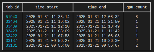
It should be noted that we collect GPU usage information every 3 - 3.5 hours. If you have recently submitted a job, your job may not be available yet.
Link to section 'Inspecting a specific job' of 'GPU Usage Monitoring' Inspecting a specific job
If you want to view the GPU utilization of a specific job, you can use the -j or --job_id flag. For example, to see the utilization of job 32083, you may run the following:
/apps/external/gpu_util/get_gpu_util --job_id 32083
This will print a table of the GPU memory and utilization for each GPU that was allocated for the specified job:
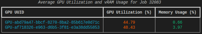
Link to section 'Plotting Data' of 'GPU Usage Monitoring' Plotting Data
It is also possible to plot the GPU utilization and memory usage over time with the -p or the --plot flag:
/apps/external/gpu_util/get_gpu_util --job_id 32083 --plot
This will print two graphs. The first will be a 2-minute rolling average of the GPU utilization over time, and the second will be the percentage of memory used over time. Each GPU will be colored differently:
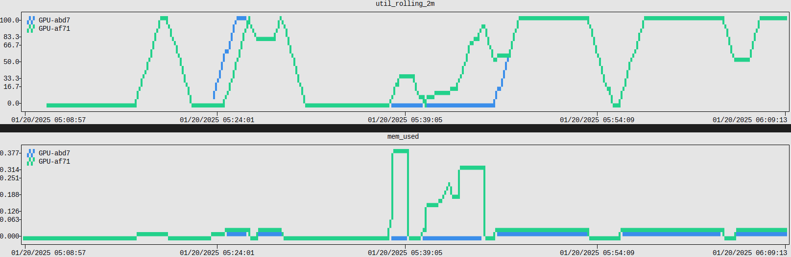
Link to section 'Saving GPU Data' of 'GPU Usage Monitoring' Saving GPU Data
If you would like to save the raw GPU utilization and memory usage data for your job, you can use the -s or --save flag:
/apps/external/gpu_util/get_gpu_util --job_id 32083 --save
This will download the GPU data for a specific job as:
{job_id}_gpu_usage.csv
Link to section 'Checking Account Usage (Group Managers only)' of 'GPU Usage Monitoring' Checking Account Usage (Group Managers only)
If you are a manager of a specific group, you are able to query all accounts owned by that group. You can check the usage of all members of your account over the previous week by running:
/apps/external/gpu_util/get_gpu_util -A accountnameIf you would like a breakdown of the individual jobs ran within the past week, you can add the --records flag:
/apps/external/gpu_util/get_gpu_util -A accountname --recordsFurther, the --job {jobid} flag will also allow you to query the utilization of individual jobs that were ran on an account that you manage.
Link to section 'FAQ/Troubleshooting' of 'GPU Usage Monitoring' FAQ/Troubleshooting
- "Why doesn't my job show up in the list?"
- Although we log GPU utilization every 10 seconds, we only actually collect it every 3-3.5 hours. If you check later, your job should be listed.
- "Can other people see my data?"
- No, our interface only allows users to check the utilization of their own jobs.
- "Is this a good way to see the GPU Hours balance?"
- No, the primary purpose of this tool is to check that GPUs are actually being used, not to track billed GPU hours. To see the total GPU hours balance, please use the
slistcommand.
- No, the primary purpose of this tool is to check that GPUs are actually being used, not to track billed GPU hours. To see the total GPU hours balance, please use the