Case Calculating with Fluent
Link to section 'Calculation with Fluent' of 'Case Calculating with Fluent' Calculation with Fluent
Now all the files are ready for the Fluent calculations. Both “Geometry” and “Mesh” cells should have green checks. We can set up the CFD simulation parameters in the Ansys Fluent by double-clicking the “Setup” cell.
Ansys Fluent Launcher can be started by selecting “editing” on the “Setup” cell with many startup options (e.g. Precision, Parallel, Display). Note that “Dimension” is fixed to “3D” because we are using a 3D model in this project.
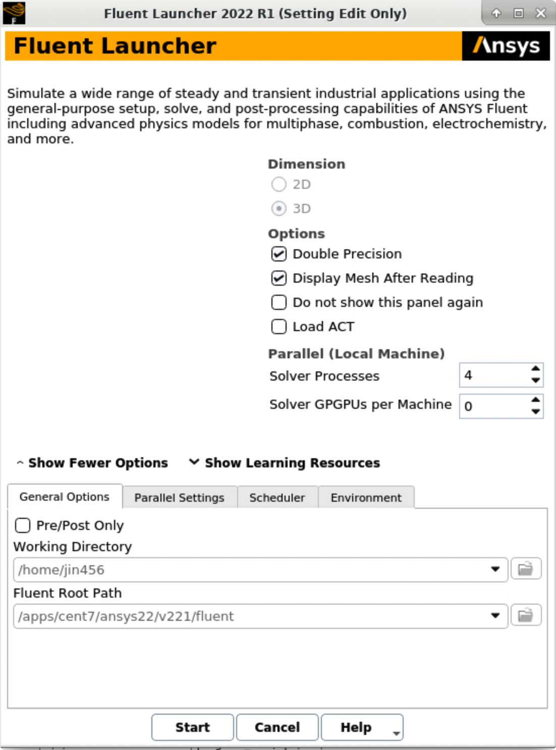
After the Fluent is opened, an Ansys Fluent settings file FFF.set is written under the folder $Ansys_PROJECT_FOLDER/elbow_demo_file/dp0/FFF/Fluent/.
Then we are going to set up all the necessary parameters for Fluent computation. Here are the key steps for the setup:
- Setting up the domain:
- Change the units for length to be consistent with the Mesh;
- Check the mesh statistics and quality;
- Setting up physics:
- Solver: “Energy”, “Viscous Model”, “Near-Wall Treatment”;
- Materials;
- Zones;
- Boundaries: Inlet, Outlet, Internal, Symmetry, Wall;
- Solving:
- Solution Methods;
- Reports;
- Initialization;
- Iterations and output frequency.
Then the calculation will be carried out and the results will be written out into FFF-1.cas.gz under folder $Ansys_PROJECT_FOLDER/elbow_demo_file/dp0/FFF/Fluent/.
This file contains all the settings and simulation results which can be loaded for post analysis and re-computation (more details will be introduced in the following sections). If only configurations and settings within the Fluent are needed, we can open independent Fluent or submit Fluent jobs with bash commands by loading the existing case in order to facilitate the computation process.
Parameters used in demo case (use default if not assigned):
- Domain Setup: Length Units=”mm”;
- Solver: Energy=”on”; Viscous Model=”k-epsilon”; Near-Wall Treatment=”Enhanced Wall Treatment”;
- Materials: water (Density=1000[kg/m^3]; Specific Heat=4216[J/kg-k]; Thermal Conductivity=0.677[w/m-k]; Viscosity=8e-4[kg/m-s]);
- Zones=”fluid (water)”;
- Inlet=”velocity-inlet-large” (Velocity Magnitude=0.4m/s, Specification Method=”Intensity and Hydraulic Diameter”, Turbulent Intensity=5%; Hydraulic Diameter=100mm; Thermal Temperature=293.15k) &”velocity-inlet-small” (Velocity Magnitude=1.2m/s, Specification Method=”Intensity and Hydraulic Diameter”, Turbulent Intensity=5%; Hydraulic Diameter=25mm; Thermal Temperature=313.15k); Internal=”interior-fluid”; Symmetry=”symmetry”; Wall=”wall-fluid”;
- Solution Methods: Gradient=”Green-Gauss Node Based”;
- Report: plot residual and “Facet Maximum” for “pressure-outlet”
- Hybrid Initialization;
- 300 iterations.
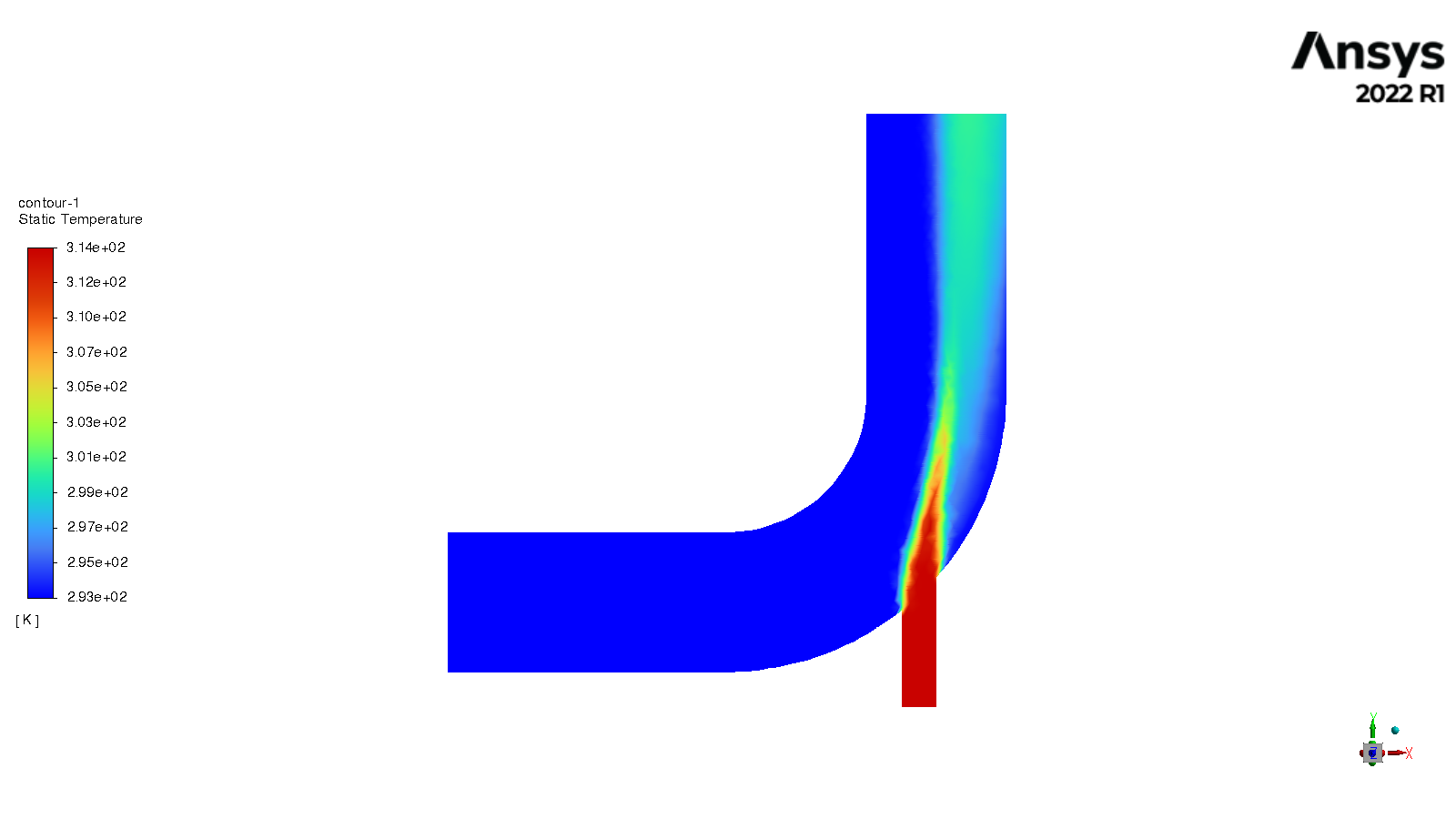
Link to section 'Results analysis' of 'Case Calculating with Fluent' Results analysis
The best methods to view and analyze the simulation should be the Ansys Fluent (directly after computation) or the Ansys CFD-Post (entering “Results” in Ansys Workbench). Both methods are straightforward so we will not cover this part in this tutorial. Here is a final simulation result showing the temperature of the symmetry after 300 iterations for reference: