Purdue University

Preparing Case Files for Fluent

Link to section 'Creating a Fluent fluid analysis system' of 'Preparing Case Files for Fluent' Creating a Fluent fluid analysis system

In the Ansys Workbench, create a new fluid flow analysis by double-clicking the Fluid Flow (Fluent) option under the Analysis Systems in the Toolbox on the left panel. You can also drag-and-drop the analysis system into the Project Schematic. A green dotted outline indicating a potential location for the new system initially appears in the Project Schematic. When you drag the system to one of the outlines, it turns into a red box to indicate the chosen location of the new system.

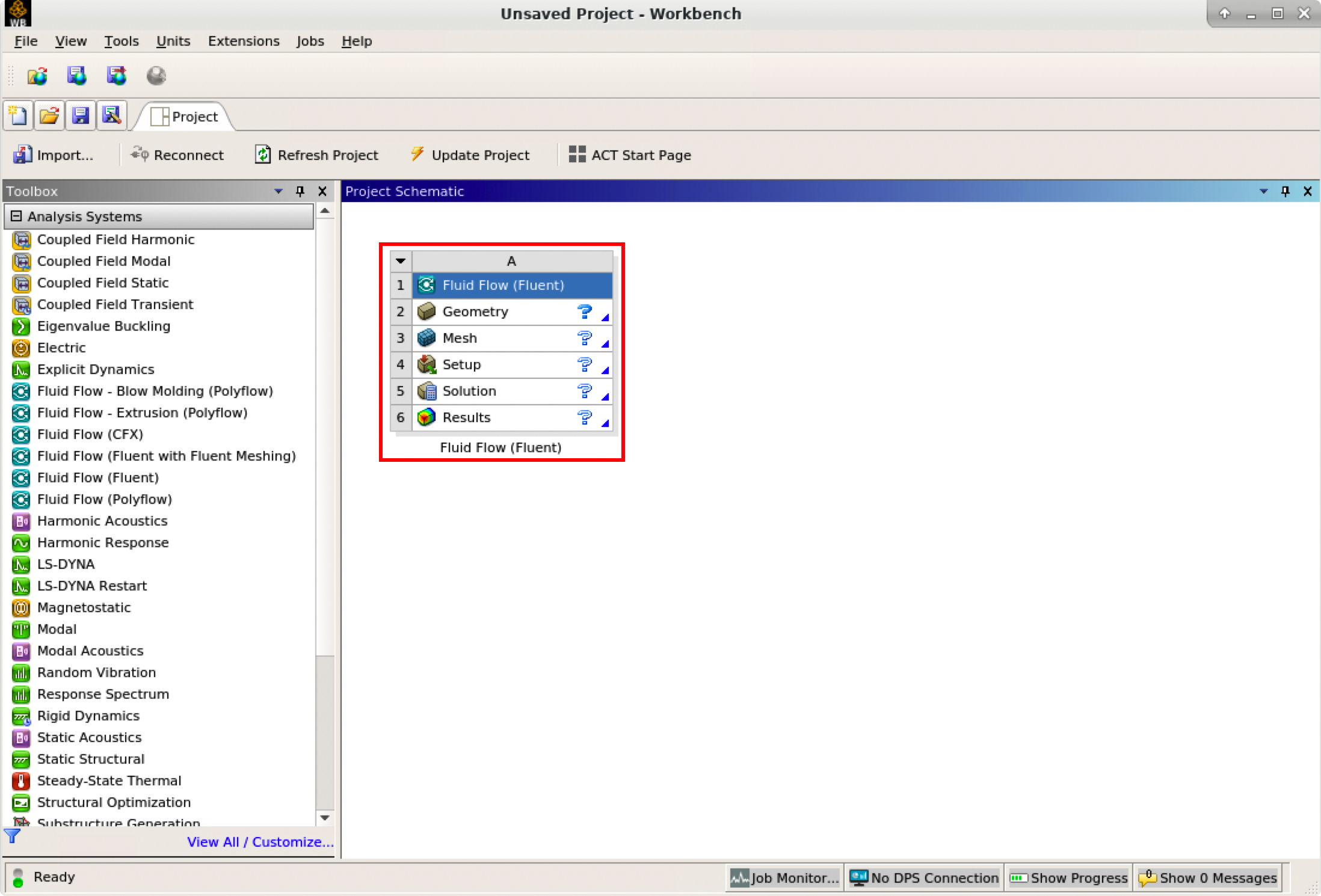
The red rectangle indicates the Fluid Flow system for Fluent, which includes all the essential workflows from “2 Geometry” to “6 Results”. You can rename it and carry out the necessary step-by-step procedures by double-clicking the corresponding cells.

It is important to save the project. Ansys Workbench saves the project with a .wbpj extension and also all the supporting files into a folder with the same name. In this case, a file named elbow_demo.wbpj and a folder $Ansys_PROJECT_FOLDER/elbow_demo_files/ are created in the Ansys project folder:

$ ll
total 33
drwxr-xr-x 7  myusername itap     9 Mar  3 17:47 elbow_demo_files
-rw-r--r-- 1  myusername itap 42597 Mar  3 17:47 elbow_demo.wbpj

You should always “Update Project” and save it after finishing a procedure.

Link to section 'Creating Geometry in the Ansys DesignModeler' of 'Preparing Case Files for Fluent' Creating Geometry in the Ansys DesignModeler

Create a geometry in the Ansys DesignModeler (by double-clicking “Geometry” cell in workflow), or import the appropriate geometry file (by right-clicking the Geometry cell and selecting “Import Geometry” option from the context menu).

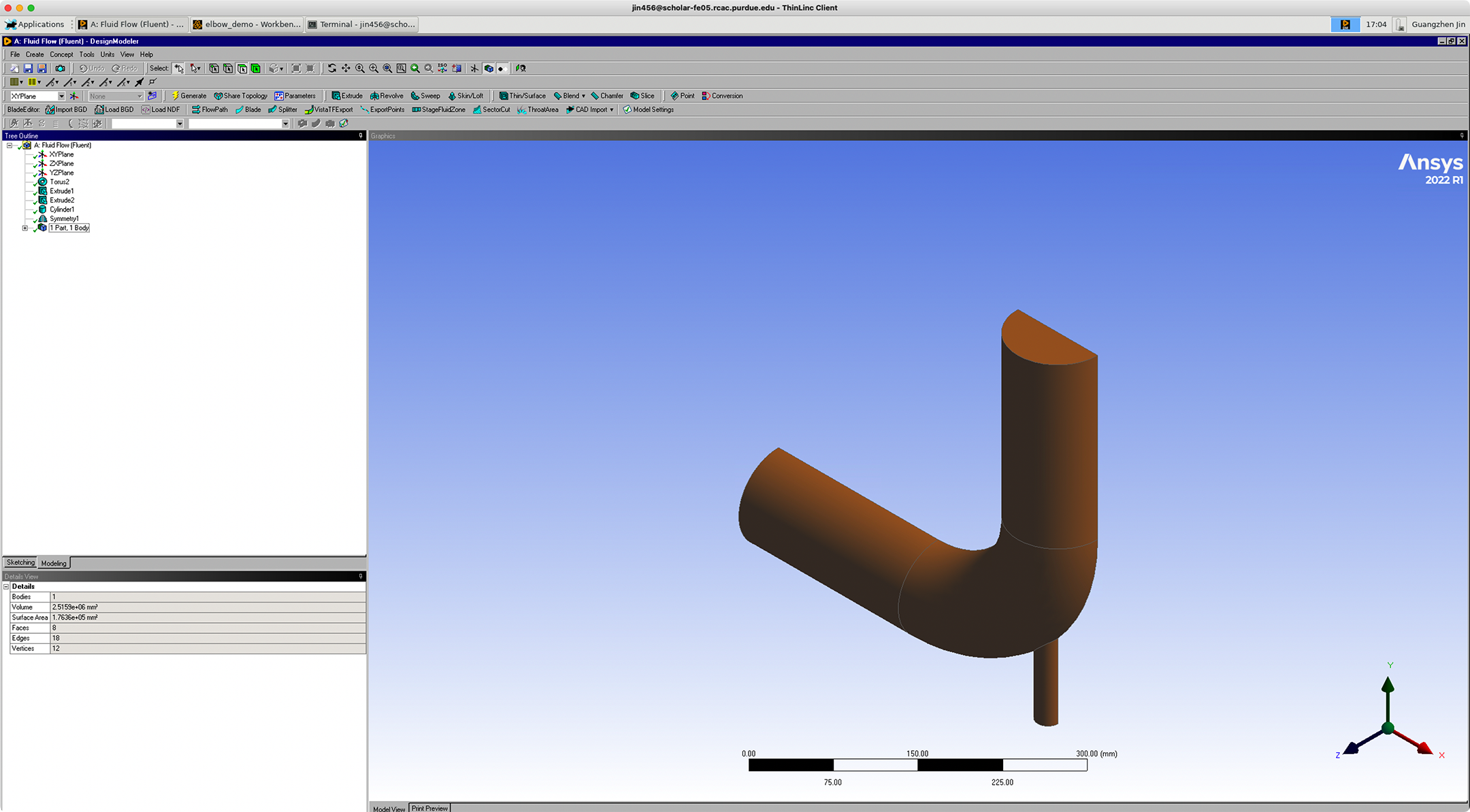
You can use Ansys DesignModeler to create 2D/3D geometries or even draw the objects yourself. In our example, we created only half of the elbow pipe because the symmetry of the structure is taken into account to reduce the computation intensity.

After saving the geometry, a geometry file FFF.agdb will be created in the folder: $Ansys_PROJECT_FOLDER/elbow_demo_file/dp0/FFF/DM/. The project in Workbench will be updated automatically.

If you import a pre-existing geometry into Ansys DesignModeler, it will also generate this file with the same filename at this location.

Link to section 'Creating mesh in the Ansys Meshing' of 'Preparing Case Files for Fluent' Creating mesh in the Ansys Meshing

Now that we have created the elbow pipe geometry, a computational mesh can be generated by the Meshing application throughout the flow volume.

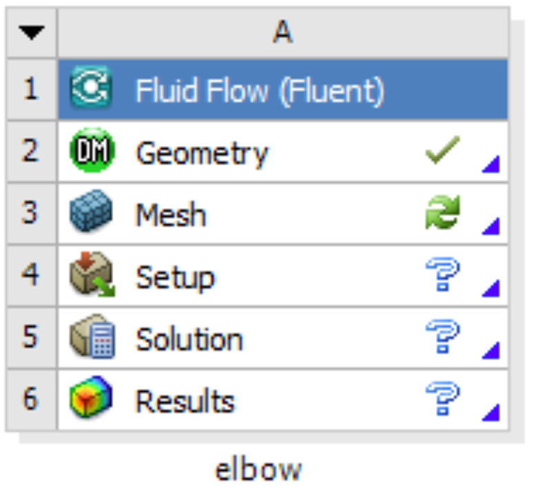
With the successful creation of the geometry, there should be a green check showing the completion of “Geometry” in the Ansys Workbench. A Refresh Required icon within the “Mesh” cell indicates the mesh needs to be updated and refreshed for the system.

Then it’s time to open the Ansys Meshing application by double-clicking the “Mesh” cell and editing the mesh for the project. Generally, there are several steps we need to take to define the mesh:

1. Create names for all geometry boundaries such as the inlets, outlets and fluid body. Note: You can use the strings “velocity inlet” and “pressure outlet” in the named selections (with or without hyphens or underscore characters) to allow Ansys Fluent to automatically detect and assign the corresponding boundary types accordingly. Use “Fluid” for the body to let Ansys Fluent automatically detect that the volume is a fluid zone and treat it accordingly.
2. Set basic meshing parameters for the Ansys Meshing application. Here are several important parameters you may need to assign: Sizing, Quality, Body Sizing Control, Inflation.
3. Select “Generate” to generate the mesh and “Update” to update the mesh into the system. Note: Once the mesh is generated, you can view the mesh statistics by opening the Statistics node in the Details of “Mesh” view. This will display information such as the number of nodes and the number of elements, which gives you a general idea for the future computational resources and time.

After generation and updating the mesh, a mesh file FFF.msh will be generated in folder $Ansys_PROJECT_FOLDER/elbow_demo_file/dp0/FFF/MECH/ and a mesh database file FFF.mshdb will be generated in folder $Ansys_PROJECT_FOLDER/elbow_demo_file/dp0/global/MECH/.

Parameters used in demo case (use default if not assigned):

1. Length Unit=”mm”
2. Names defined for geometry:
   • velocity-inlet-large (large inlet on pipe);
   • velocity-inlet-small (small inlet on pipe);
   • pressure-outlet (outlet on pipe);
   • symmetry (symmetry surface);
   • Fluid (body);
3. Mesh:
   • Quality: Smoothing=”high”;
   • Inflation: Use Automatic Inflation=“Program Controlled”, Inflation Option=”Smooth Transition”;
4. Statistics:
   • Nodes=29371;
   • Elements=87647.

Link to section 'Calculation with Fluent' of 'Preparing Case Files for Fluent' Calculation with Fluent

Now all the preparations have been ready for the numerical calculation in Ansys Fluent. Both “Geometry” and “Mesh” cells should have green checks on. We can set up the CFD simulation parameters in Ansys Fluent by double-clicking the “Setup” cell.

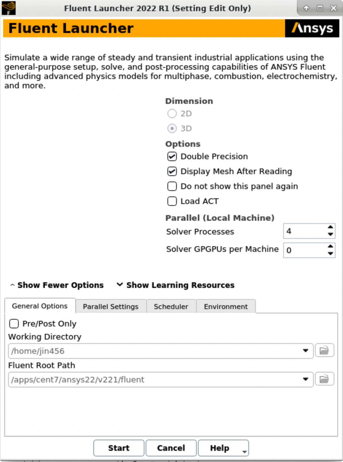
When Ansys Fluent is first started or by selecting “editing” on the “Setup” cell, the Fluent Launcher is displayed, enabling you to view and/or set certain Ansys Fluent start-up options (e.g. Precision, Parallel, Display). Note that “Dimension” is fixed to “3D” because we are using a 3D model in this project.

After the Fluent is opened, an Ansys Fluent settings file FFF.set is written under the folder $Ansys_PROJECT_FOLDER/elbow_demo_file/dp0/FFF/Fluent/.

Then we are going to set up all the necessary parameters for Fluent computation. Here are the key steps for the setup:

1. Setting up the domain:
   • Change the units for length to be consistent with the Mesh;
   • Check the mesh statistics and quality;
2. Setting up physics:
   • Solver: “Energy”, “Viscous Model”, “Near-Wall Treatment”;
   • Materials;
   • Zones;
   • Boundaries: Inlet, Outlet, Internal, Symmetry, Wall;
3. Solving:
   • Solution Methods;
   • Reports;
   • Initialization;
   • Iterations and output frequency.

Then the calculation will be carried out and the results will be written out into FFF-1.cas.gz under folder $Ansys_PROJECT_FOLDER/elbow_demo_file/dp0/FFF/Fluent/.

This file contains all the settings and simulation results which can be loaded for post analysis and re-computation (more details will be introduced in the following sections). If only configurations and settings within the Fluent are needed, we can open independent Fluent or submit Fluent jobs with bash commands by loading the existing case in order to facilitate the computation process.

Parameters used in demo case (use default if not assigned):

1. Domain Setup: Length Units=”mm”;
2. Solver: Energy=”on”; Viscous Model=”k-epsilon”; Near-Wall Treatment=”Enhanced Wall Treatment”;
3. Materials: water (Density=1000[kg/m^3]; Specific Heat=4216[J/kg-k]; Thermal Conductivity=0.677[w/m-k]; Viscosity=8e-4[kg/m-s]);
4. Zones=”fluid (water)”;
5. Inlet=”velocity-inlet-large” (Velocity Magnitude=0.4m/s, Specification Method=”Intensity and Hydraulic Diameter”, Turbulent Intensity=5%; Hydraulic Diameter=100mm; Thermal Temperature=293.15k) &”velocity-inlet-small” (Velocity Magnitude=1.2m/s, Specification Method=”Intensity and Hydraulic Diameter”, Turbulent Intensity=5%; Hydraulic Diameter=25mm; Thermal Temperature=313.15k); Internal=”interior-fluid”; Symmetry=”symmetry”; Wall=”wall-fluid”;
6. Solution Methods: Gradient=”Green-Gauss Node Based”;
7. Report: plot residual and “Facet Maximum” for “pressure-outlet”
8. Hybrid Initialization;
9. 300 iterations.

Case Calculating with Fluent

Link to section 'Calculation with Fluent' of 'Case Calculating with Fluent' Calculation with Fluent

Now all the files are ready for the Fluent calculations. Both “Geometry” and “Mesh” cells should have green checks. We can set up the CFD simulation parameters in the Ansys Fluent by double-clicking the “Setup” cell.

Ansys Fluent Launcher can be started by selecting “editing” on the “Setup” cell with many startup options (e.g. Precision, Parallel, Display). Note that “Dimension” is fixed to “3D” because we are using a 3D model in this project.

After the Fluent is opened, an Ansys Fluent settings file FFF.set is written under the folder $Ansys_PROJECT_FOLDER/elbow_demo_file/dp0/FFF/Fluent/.

Then we are going to set up all the necessary parameters for Fluent computation. Here are the key steps for the setup:

1. Setting up the domain:
   • Change the units for length to be consistent with the Mesh;
   • Check the mesh statistics and quality;
2. Setting up physics:
   • Solver: “Energy”, “Viscous Model”, “Near-Wall Treatment”;
   • Materials;
   • Zones;
   • Boundaries: Inlet, Outlet, Internal, Symmetry, Wall;
3. Solving:
   • Solution Methods;
   • Reports;
   • Initialization;
   • Iterations and output frequency.

Then the calculation will be carried out and the results will be written out into FFF-1.cas.gz under folder $Ansys_PROJECT_FOLDER/elbow_demo_file/dp0/FFF/Fluent/.

This file contains all the settings and simulation results which can be loaded for post analysis and re-computation (more details will be introduced in the following sections). If only configurations and settings within the Fluent are needed, we can open independent Fluent or submit Fluent jobs with bash commands by loading the existing case in order to facilitate the computation process.

Parameters used in demo case (use default if not assigned):

1. Domain Setup: Length Units=”mm”;
2. Solver: Energy=”on”; Viscous Model=”k-epsilon”; Near-Wall Treatment=”Enhanced Wall Treatment”;
3. Materials: water (Density=1000[kg/m^3]; Specific Heat=4216[J/kg-k]; Thermal Conductivity=0.677[w/m-k]; Viscosity=8e-4[kg/m-s]);
4. Zones=”fluid (water)”;
5. Inlet=”velocity-inlet-large” (Velocity Magnitude=0.4m/s, Specification Method=”Intensity and Hydraulic Diameter”, Turbulent Intensity=5%; Hydraulic Diameter=100mm; Thermal Temperature=293.15k) &”velocity-inlet-small” (Velocity Magnitude=1.2m/s, Specification Method=”Intensity and Hydraulic Diameter”, Turbulent Intensity=5%; Hydraulic Diameter=25mm; Thermal Temperature=313.15k); Internal=”interior-fluid”; Symmetry=”symmetry”; Wall=”wall-fluid”;
6. Solution Methods: Gradient=”Green-Gauss Node Based”;
7. Report: plot residual and “Facet Maximum” for “pressure-outlet”
8. Hybrid Initialization;
9. 300 iterations.

Link to section 'Results analysis' of 'Case Calculating with Fluent' Results analysis

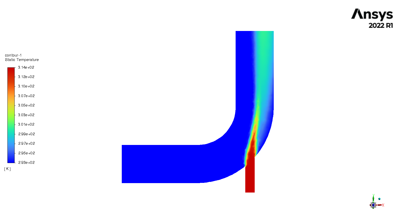
The best methods to view and analyze the simulation should be the Ansys Fluent (directly after computation) or the Ansys CFD-Post (entering “Results” in Ansys Workbench). Both methods are straightforward so we will not cover this part in this tutorial. Here is a final simulation result showing the temperature of the symmetry after 300 iterations for reference:

Fluent Text User Interface and Journal File

Link to section 'Fluent Text User Interface (TUI)' of 'Fluent Text User Interface and Journal File' Fluent Text User Interface (TUI)

If you pay attention to the “Console” window in the Fluent window when setting up and carrying out the calculation, corresponding commands can be found and executed one after another. Almost all the setting processes can be accomplished by the command lines, which is called Fluent Text User Interface (TUI). Here are the main commands in Fluent TUI:

  adjoint/                parallel/               solve/
  define/                 plot/                   surface/
  display/                preferences/            turbo-workflow/
  exit                    print-license-usage     views/
  file/                   report/
  mesh/                   server/

For example, instead of opening a case by clicking buttons in Ansys Fluent, we can type /file read-case case_file_name.cas.gz to open the saved case.

Link to section 'Fluent Journal Files' of 'Fluent Text User Interface and Journal File' Fluent Journal Files

A Fluent journal file is a series of TUI commands stored in a text file. The file can be written in a text editor or generated by Fluent as a transcript of the commands given to Fluent during your session.

A journal file generated by Fluent will include any GUI operations (in a TUI form, though). This is quite useful if you have a series of tasks that you need to execute, as it provides a shortcut. To record a journal file, start recording with File -> Write -> Start Journal..., perform whatever tasks you need, and then stop recording with File -> Write -> Stop Journal...

You can also write your own journal file into a text file. The basic rule for a Fluent journal file is to reproduce the TUI commands that controlled the configuration and calculation of Fluent in their order. You can add a comment in a line starting with a ; (semicolon).

Here are some reasons why you should use a Fluent journal file:

1. Using journal files with bash scripting can allow you to automate your jobs.
2. Using journal files can allow you to parameterize your models easily and automatically.
3. Using a journal file can set parameters you do not have in your case file e.g. autosaving.
4. Using a journal file can allow you to safely save, stop and restart your jobs easily.

The order of your journal file commands is highly important. The correct sequences must be followed and some stages have multiple options e.g. different initialization methods.

Here is a sample Fluent journal file for the demo case:

  ;testJournal.jou
  ;Set the TUI version for Fluent
  /file/set-tui-version "22.1"
  ;Read the case. The default folder
  /file read-case /home/jin456/Fluent_files/tutorial_case1/elbow_files/dp0/FFF/Fluent/FFF-1.cas.gz
  ;Initialize the case with Hybrid Initialization
  /solve/initialize/hyb-initialization
  ;Set Number of Iterations to 1000, Reporting Interval to 10 iterations and Profile Update Interval to 1 iteration
  /solve/iterate 1000 10 1
  ;Outputting solver performance data upon completion of the simulation
  /parallel timer usage
  ;Write out the simulation results.
  /file write-case-data /home/jin456/Fluent_files/tutorial_case1/elbow_files/dp0/FFF/Fluent/result.cas.h5
  ;After computation, exit Flent
  /exit

Before running this Fluent journal file, you need to make sure: 1) the ansys module has been loaded (it’s highly recommended to load the same version of Ansys when you built the case project); 2) the project case file (***.cas.gz) has been created.

Then we can use Fluent to run this journal file by simply using:fluent 3ddp -t$NTASKS -g -i testJournal.jou in the terminal. Here, 3d indicates this is a 3d model, dp indicates double precision, -t$NTASKS tells Fluent how many Solver Processes it will take (e.g. -t4), -g means to run without the GUI or graphics, -i testJournal.jou tells Fluent to read the specific journal file.

Here is a table for the available command line Options for Linux/UNIX and Windows Platforms in Ansys Fluent.

For more information for Fluent text user interface and journal files, please refer to Fluent FAQ.

Submitting Fluent jobs to SLURM

The Fluent simulations can also run in batch. In this section we provide an example script for submitting Fluent jobs to the SLURM scheduler. Please refer to the Running Jobs section of our user guide for detailed tutorials of submitting jobs.

#!/bin/bash
# Job script for submitting a FLUENT job on multiple cores on a single node 

# Apply resources via SLURM
#SBATCH --nodes=1
#SBATCH --ntasks=4
#SBATCH --time=01:00:00
#SBATCH --job-name=fluent_test
#SBATCH -o fluent_test_%j.out
#SBATCH -e fluent_test_%j.err

# Loads Ansys and sets the application up
module purge
module load ansys/2022R1

#Initiating Fluent and reading input journal file
fluent 3ddp -t$NTASKS -g -i testJournal.jou