
Scholar User Guide
Scholar is a small computer cluster, suitable for classroom learning about high performance computing (HPC).
Link to section 'Overview of Scholar' of 'Overview of Scholar' Overview of Scholar
Scholar is a small computer cluster, suitable for classroom learning about high performance computing (HPC). It consists of 6 interactive login servers and 16 batch worker nodes.
It can be accessed as a typical cluster, with a job scheduler distributing batch jobs onto its worker nodes, or as an interactive resource, with software packages available through a desktop-like environment on its login servers.
If you have a class that you think will benefit from the use of Scholar, you can schedule it for your class through our Class Account Request page. You only need to register your class itself. All students who register for the class will automatically get login privileges to the Scholar cluster.
As a batch resource, the cluster has access to typical HPC software packages and tool chains; as an interactive resource, Scholar provides a Linux remote desktop, or a Jupyter notebook server, or an R Studio server. Jupyter and R Studio can be used by students without any reliance on Linux knowledge or experience.
Link to section 'Scholar Specifications' of 'Overview of Scholar' Scholar Specifications
| Front-Ends | Number of Nodes | Processors per Node | Cores per Node | Memory per Node | Retires in |
|---|---|---|---|---|---|
| No GPU | 3 | Two AMD EPYC 9634 ("Genoa") 84-Core Processors | 168 | 384 GB | 2029 |
| With GPU | 3 | Two Intel Xeon Gold 6126 ("Skylake") 12-Core Processors with one NVIDIA Tesla V100 32GB GPU | 24 | 768 GB | 2027 |
| Sub-Cluster | Number of Nodes | Processors per Node | Cores per Node | Memory per Node | Retires in |
|---|---|---|---|---|---|
| A | 4 | Two AMD EPYC 7713 ("Milan") 64-Core Processors | 128 | 256 GB | 2027 |
| B | 3 | One AMD EPYC 7702P ("Rome") 64-Core Processor | 64 | 256 GB | 2026 |
| G | 4 | Two Intel Xeon Silver 4110 ("Skylake") 8-Core Processors with one NVIDIA Tesla V100 16GB GPU | 16 | 192 GB | 2027 |
| H | 2 | Two AMD EPYC 7543 3rd generation ("Milan") 32-Core Processors with two NVIDIA A30 24GB GPUs | 64 | 512 GB | 2027 |
| H-MIG | 2 | Two AMD EPYC 7543 3rd generation ("Milan") 32-Core Processors with eight 6GB Multi-Instance GPUs (MIGs) configured from two NVIDIA A30 24GB GPUs. | 64 | 512 GB | 2027 |
| I-MIG | 1 | Two AMD EPYC 9554 ("Genoa") 64-Core Processors with four 6GB Multi-Instance GPUs (MIGs) configured from one NVIDIA A30 24GB GPU | 128 | 384 GB | 2029 |
| J | 4 | Two Intel Xeon Gold 6126 ("Skylake") 12-Core Processors with two NVIDIA A40 48GB GPUs | 24 | 192 GB | 2029 |
Faculty who would like to know more about Scholar, please read the Faculty Guide
Link to section 'Software catalog' of 'Overview of Scholar' Software catalog
Link to section 'Accounts on Scholar' of 'Accounts' Accounts on Scholar
Link to section 'Obtaining an Account' of 'Accounts' Obtaining an Account
All Purdue faculty may request access to Scholar for use in the classroom. Please use the Accounts for Classes tool to create accounts for your class. You will need to select the semester and CRN of the class. All students registered in that class will be added once the request is fulfilled. You may add additional instructors or TAs from the same tool.
Link to section 'Outside Collaborators' of 'Accounts' Outside Collaborators
A valid Purdue Career Account is required for access to any resource. If you do not currently have a valid Purdue Career Account you must have a current Purdue faculty or staff member file a Request for Privileges (R4P) before you can proceed.
Logging In
To submit jobs on Scholar, log in to the submission host scholar.rcac.purdue.edu via SSH. This submission host is actually 7 front-end hosts: scholar-fe00 through scholar-fe06 The login process randomly assigns one of these front-ends to each login to scholar.rcac.purdue.edu.
To submit jobs on Scholar front ends with local GPUs, log in to gpu.scholar.rcac.purdue.edu via SSH.
Purdue Login
Link to section 'SSH' of 'Purdue Login' SSH
- SSH to the cluster as usual.
- When asked for a password, type your password followed by "
,push". - Your Purdue Duo client will receive a notification to approve the login.
Link to section 'Thinlinc' of 'Purdue Login' Thinlinc
- When asked for a password, type your password followed by "
,push". - Your Purdue Duo client will receive a notification to approve the login.
- The native Thinlinc client will prompt for Duo approval twice due to the way Thinlinc works.
- The native Thinlinc client also supports key-based authentication.
Passwords
Scholar supports either Purdue two-factor authentication (Purdue Login) or SSH keys.
SSH Client Software
Secure Shell or SSH is a way of establishing a secure connection between two computers. It uses public-key cryptography to authenticate the user with the remote computer and to establish a secure connection. Its usual function involves logging in to a remote machine and executing commands. There are many SSH clients available for all operating systems:
Linux / Solaris / AIX / HP-UX / Unix:
- The
sshcommand is pre-installed. Log in usingssh myusername@scholar.rcac.purdue.edufrom a terminal.
Microsoft Windows:
- MobaXterm is a small, easy to use, full-featured SSH client. It includes X11 support for remote displays, SFTP capabilities, and limited SSH authentication forwarding for keys.
Mac OS X:
- The
sshcommand is pre-installed. You may start a local terminal window from "Applications->Utilities". Log in by typing the commandssh myusername@scholar.rcac.purdue.edu.
When prompted for password, enter your Purdue career account password followed by ",push ". Your Purdue Duo client will then receive a notification to approve the login.
SSH Keys
Link to section 'General overview' of 'SSH Keys' General overview
To connect to Scholar using SSH keys, you must follow three high-level steps:
- Generate a key pair consisting of a private and a public key on your local machine.
- Copy the public key to the cluster and append it to
$HOME/.ssh/authorized_keysfile in your account. - Test if you can ssh from your local computer to the cluster without using your Purdue password.
Detailed steps for different operating systems and specific SSH client softwares are give below.
Link to section 'Mac and Linux:' of 'SSH Keys' Mac and Linux:
-
Run
ssh-keygenin a terminal on your local machine. You may supply a filename and a passphrase for protecting your private key, but it is not mandatory. To accept the default settings, press Enter without specifying a filename.
Note: If you do not protect your private key with a passphrase, anyone with access to your computer could SSH to your account on Scholar. -
By default, the key files will be stored in
~/.ssh/id_rsaand~/.ssh/id_rsa.pubon your local machine. -
Copy the contents of the public key into
$HOME/.ssh/authorized_keyson the cluster with the following command. When asked for a password, type your password followed by ",push". Your Purdue Duo client will receive a notification to approve the login.ssh-copy-id -i ~/.ssh/id_rsa.pub myusername@scholar.rcac.purdue.eduNote: use your actual Purdue account user name.
If your system does not have the
ssh-copy-idcommand, use this instead:cat ~/.ssh/id_rsa.pub | ssh myusername@scholar.rcac.purdue.edu "mkdir -p ~/.ssh && chmod 700 ~/.ssh && cat >> ~/.ssh/authorized_keys" -
Test the new key by SSH-ing to the server. The login should now complete without asking for a password.
-
If the private key has a non-default name or location, you need to specify the key by
ssh -i my_private_key_name myusername@scholar.rcac.purdue.edu
Link to section 'Windows:' of 'SSH Keys' Windows:
| Programs | Instructions |
|---|---|
| MobaXterm | Open a local terminal and follow Linux steps |
| Git Bash | Follow Linux steps |
| Windows 10 PowerShell | Follow Linux steps |
| Windows 10 Subsystem for Linux | Follow Linux steps |
| PuTTY | Follow steps below |
PuTTY:
-
Launch PuTTYgen, keep the default key type (RSA) and length (2048-bits) and click Generate button.
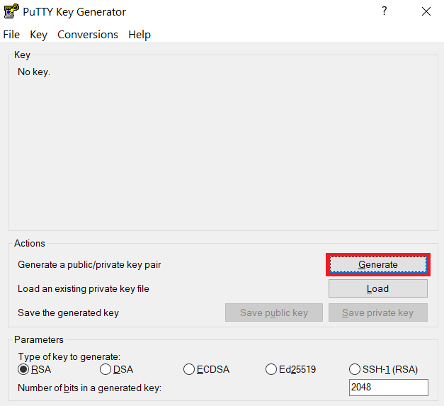
The "Generate" button can be found under the "Actions" section of the PuTTY Key Generator interface. -
Once the key pair is generated:
Use the Save public key button to save the public key, e.g.
Documents\SSH_Keys\mylaptop_public_key.pubUse the Save private key button to save the private key, e.g.
Documents\SSH_Keys\mylaptop_private_key.ppk. When saving the private key, you can also choose a reminder comment, as well as an optional passphrase to protect your key, as shown in the image below. Note: If you do not protect your private key with a passphrase, anyone with access to your computer could SSH to your account on Scholar.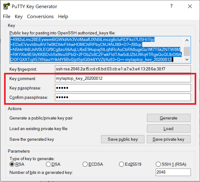
The PuTTY Key Generator form has inputs for the Key passphrase and optional reminder comment. From the menu of PuTTYgen, use the "Conversion -> Export OpenSSH key" tool to convert the private key into openssh format, e.g.
Documents\SSH_Keys\mylaptop_private_key.opensshto be used later for Thinlinc. -
Configure PuTTY to use key-based authentication:
Launch PuTTY and navigate to "Connection -> SSH ->Auth" on the left panel, click Browse button under the "Authentication parameters" section and choose your private key, e.g. mylaptop_private_key.ppk
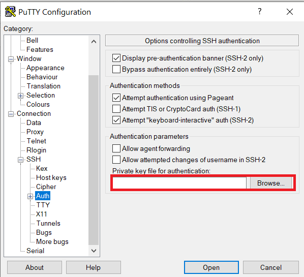
After clicking Connection -> SSH ->Auth panel, the "Browse" option can be found at the bottom of the resulting panel. Navigate back to "Session" on the left panel. Highlight "Default Settings" and click the "Save" button to ensure the change in place.
-
Connect to the cluster. When asked for a password, type your password followed by "
,push". Your Purdue Duo client will receive a notification to approve the login. Copy the contents of public key from PuTTYgen as shown below and paste it into$HOME/.ssh/authorized_keys. Please double-check that your text editor did not wrap or fold the pasted value (it should be one very long line).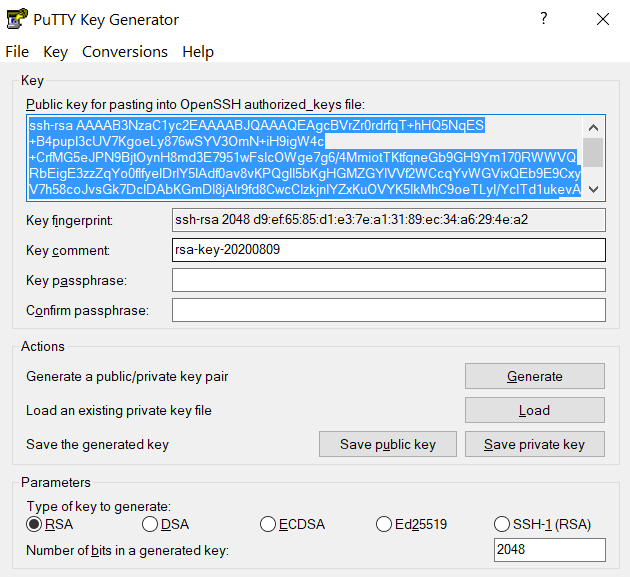
The "Public key" will look like a long string of random letters and numbers in a text box at the top of the window. - Test by connecting to the cluster. If successful, you will not be prompted for a password or receive a Duo notification. If you protected your private key with a passphrase in step 2, you will instead be prompted to enter your chosen passphrase when connecting.
ThinLinc
RCAC provides Cendio's ThinLinc as an alternative to running an X11 server directly on your computer. It allows you to run graphical applications or graphical interactive jobs directly on Scholar through a persistent remote graphical desktop session.
ThinLinc is a service that allows you to connect to a persistent remote graphical desktop session. This service works very well over a high latency, low bandwidth, or off-campus connection compared to running an X11 server locally. It is also very helpful for Windows users who do not have an easy to use local X11 server, as little to no set up is required on your computer.
There are two ways in which to use ThinLinc: preferably through the native client or through a web browser.
Link to section 'Installing the ThinLinc native client' of 'ThinLinc' Installing the ThinLinc native client
The native ThinLinc client will offer the best experience especially over off-campus connections and is the recommended method for using ThinLinc. It is compatible with Windows, Mac OS X, and Linux.
- Download the ThinLinc client from the ThinLinc website.
- Start the ThinLinc client on your computer.
- In the client's login window, use desktop.scholar.rcac.purdue.edu as the Server. Use your Purdue Career Account username and password, but append "
,push" to your password. - Click the Connect button.
- Your Purdue Login Duo will receive a notification to approve your login.
- Continue to following section on connecting to Scholar from ThinLinc.
Link to section 'Using ThinLinc through your web browser' of 'ThinLinc' Using ThinLinc through your web browser
The ThinLinc service can be accessed from your web browser as a convenience to installing the native client. This option works with no set up and is a good option for those on computers where you do not have privileges to install software. All that is required is an up-to-date web browser. Older versions of Internet Explorer may not work.
- Open a web browser and navigate to desktop.scholar.rcac.purdue.edu.
- Log in with your Purdue Career Account username and password, but append "
,push" to your password. - You may safely proceed past any warning messages from your browser.
- Your Purdue Login Duo will receive a notification to approve your login.
- Continue to the following section on connecting to Scholar from ThinLinc.
Link to section 'Connecting to Scholar from ThinLinc' of 'ThinLinc' Connecting to Scholar from ThinLinc
- Once logged in, you will be presented with a remote Linux desktop running directly on a cluster front-end.
- Open the terminal application on the remote desktop.
- Once logged in to the Scholar head node, you may use graphical editors, debuggers, software like Matlab, or run graphical interactive jobs. For example, to test the X forwarding connection issue the following command to launch the graphical editor gedit:
$ gedit - This session will remain persistent even if you disconnect from the session. Any interactive jobs or applications you left running will continue running even if you are not connected to the session.
Link to section 'Tips for using ThinLinc native client' of 'ThinLinc' Tips for using ThinLinc native client
- To exit a full screen ThinLinc session press the F8 key on your keyboard (fn + F8 key for Mac users) and click to disconnect or exit full screen.
- Full screen mode can be disabled when connecting to a session by clicking the Options button and disabling full screen mode from the Screen tab.
Link to section 'Configure ThinLinc to use SSH Keys' of 'ThinLinc' Configure ThinLinc to use SSH Keys
- The web client does NOT support public-key authentication.
-
ThinLinc native client supports the use of an SSH key pair. For help generating and uploading keys to the cluster, see SSH Keys section in our user guide for details.
To set up SSH key authentication on the ThinLinc client:
-
Open the Options panel, and select Public key as your authentication method on the Security tab.
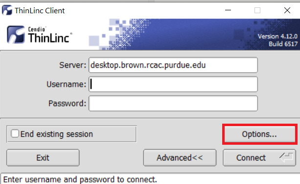
The "Options..." button in the ThinLinc Client can be found towards the bottom left, above the "Connect" button. -
In the options dialog, switch to the "Security" tab and select the "Public key" radio button:
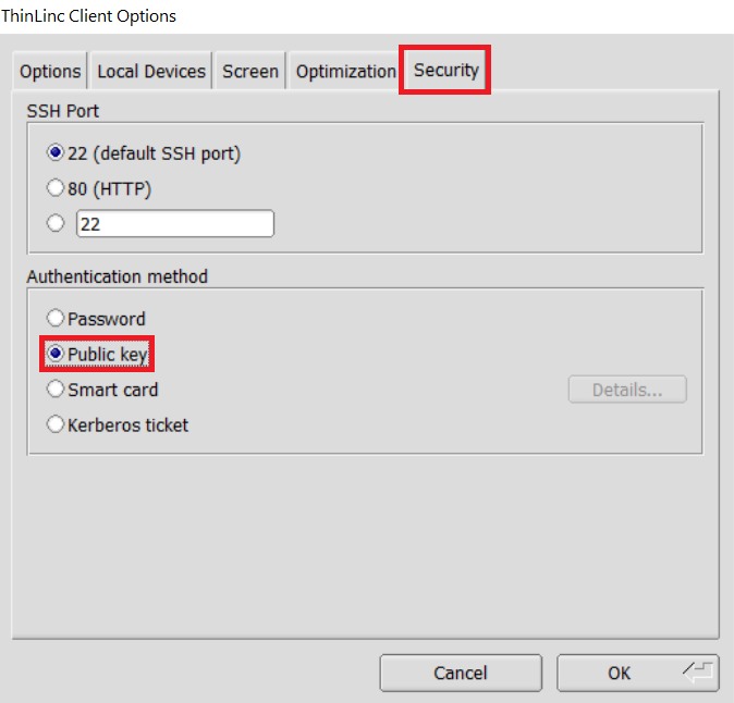
The "Security" tab found in the options dialog, will be the last of available tabs. The "Public key" option can be found in the "Authentication method" options group. - Click OK to return to the ThinLinc Client login window. You should now see a Key field in place of the Password field.
-
In the Key field, type the path to your locally stored private key or click the ... button to locate and select the key on your local system. Note: If PuTTY is used to generate the SSH Key pairs, please choose the private key in the openssh format.
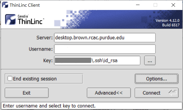
The ThinLinc Client login window will now display key field instead of a password field.
-
SSH X11 Forwarding
SSH supports tunneling of X11 (X-Windows). If you have an X11 server running on your local machine, you may use X11 applications on remote systems and have their graphical displays appear on your local machine. These X11 connections are tunneled and encrypted automatically by your SSH client.
Link to section 'Installing an X11 Server' of 'SSH X11 Forwarding' Installing an X11 Server
To use X11, you will need to have a local X11 server running on your personal machine. Both free and commercial X11 servers are available for various operating systems.
Linux / Solaris / AIX / HP-UX / Unix:
- An X11 server is at the core of all graphical sessions. If you are logged in to a graphical environment on these operating systems, you are already running an X11 server.
- ThinLinc is an alternative to running an X11 server directly on your Linux computer. ThinLinc is a service that allows you to connect to a persistent remote graphical desktop session.
Microsoft Windows:
- ThinLinc is an alternative to running an X11 server directly on your Windows computer. ThinLinc is a service that allows you to connect to a persistent remote graphical desktop session.
- MobaXterm is a small, easy to use, full-featured SSH client. It includes X11 support for remote displays, SFTP capabilities, and limited SSH authentication forwarding for keys.
Mac OS X:
- X11 is available as an optional install on the Mac OS X install disks prior to 10.7/Lion. Run the installer, select the X11 option, and follow the instructions. For 10.7+ please download XQuartz.
- ThinLinc is an alternative to running an X11 server directly on your Mac computer. ThinLinc is a service that allows you to connect to a persistent remote graphical desktop session.
Link to section 'Enabling X11 Forwarding in your SSH Client' of 'SSH X11 Forwarding' Enabling X11 Forwarding in your SSH Client
Once you are running an X11 server, you will need to enable X11 forwarding/tunneling in your SSH client:
ssh: X11 tunneling should be enabled by default. To be certain it is enabled, you may usessh -Y.- MobaXterm: Select "New session" and "SSH." Under "Advanced SSH Settings" check the box for X11 Forwarding.
SSH will set the remote environment variable $DISPLAY to "localhost:XX.YY" when this is working correctly. If you had previously set your $DISPLAY environment variable to your local IP or hostname, you must remove any set/export/setenv of this variable from your login scripts. The environment variable $DISPLAY must be left as SSH sets it, which is to a random local port address. Setting $DISPLAY to an IP or hostname will not work.
Purchasing Nodes
RCAC operates a significant shared cluster computing infrastructure developed over several years through focused acquisitions using funds from grants, faculty startup packages, and institutional sources. These "community clusters" are now at the foundation of Purdue's research cyberinfrastructure.
We strongly encourage any Purdue faculty or staff with computational needs to join this growing community and enjoy the enormous benefits this shared infrastructure provides:
- Peace of Mind
RCAC system administrators take care of security patches, attempted hacks, operating system upgrades, and hardware repair so faculty and graduate students can concentrate on research.
- Low Overhead
RCAC data centers provide infrastructure such as networking, racks, floor space, cooling, and power.
- Cost Effective
RCAC works with vendors to obtain the best price for computing resources by pooling funds from different disciplines to leverage greater group purchasing power.
Through the Community Cluster Program, Purdue affiliates have invested several million dollars in computational and storage resources from Q4 2006 to the present with great success in both the research accomplished and the money saved on equipment purchases.
For more information or to purchase access to our latest cluster today, see the Purchase page. Have questions? contact us at rcac-cluster-purchase@lists.purdue.edu to discuss.
File Storage and Transfer
Learn more about file storage transfer for Scholar.
Link to section 'Archive and Compression' of 'Archive and Compression' Archive and Compression
There are several options for archiving and compressing groups of files or directories. The mostly commonly used options are:
Link to section 'tar' of 'Archive and Compression' tar
See the official documentation for tar for more information.
Saves many files together into a single archive file, and restores individual files from the archive. Includes automatic archive compression/decompression options and special features for incremental and full backups.
Examples:
  (list contents of archive somefile.tar)
$ tar tvf somefile.tar

  (extract contents of somefile.tar)
$ tar xvf somefile.tar

  (extract contents of gzipped archive somefile.tar.gz)
$ tar xzvf somefile.tar.gz

  (extract contents of bzip2 archive somefile.tar.bz2)
$ tar xjvf somefile.tar.bz2

  (archive all ".c" files in current directory into one archive file)
$ tar cvf somefile.tar *.c

  (archive and gzip-compress all files in a directory into one archive file)
$ tar czvf somefile.tar.gz somedirectory/

  (archive and bzip2-compress all files in a directory into one archive file)
$ tar cjvf somefile.tar.bz2 somedirectory/
Other arguments for tar can be explored by using the man tar command.
Link to section 'gzip' of 'Archive and Compression' gzip
The standard compression system for all GNU software.
Examples:
  (compress file somefile - also removes uncompressed file)
$ gzip somefile

  (uncompress file somefile.gz - also removes compressed file)
$ gunzip somefile.gz
Link to section 'bzip2' of 'Archive and Compression' bzip2
See the official documentation for bzip for more information.
Strong, lossless data compressor based on the Burrows-Wheeler transform. Stronger compression than gzip.
Examples:
  (compress file somefile - also removes uncompressed file)
$ bzip2 somefile

  (uncompress file somefile.bz2 - also removes compressed file)
$ bunzip2 somefile.bz2
There are several other, less commonly used, options available as well:
- zip
- 7zip
- xz
Link to section 'Storage Environment Variables' of 'Storage Environment Variables' Storage Environment Variables
Several environment variables are automatically defined for you to help you manage your storage. Use environment variables instead of actual paths whenever possible to avoid problems if the specific paths to any of these change.
| Name | Description |
|---|---|
| HOME | /home/myusername |
| PWD | path to your current directory |
| RCAC_SCRATCH | /scratch/scholar/myusername |
By convention, environment variable names are all uppercase. You may use them on the command line or in any scripts in place of and in combination with hard-coded values:
$ ls $HOME
...

$ ls $RCAC_SCRATCH/myproject
...
To find the value of any environment variable:
$ echo $RCAC_SCRATCH
/scratch/scholar/myusername
To list the values of all environment variables:
$ env
USER=myusername
HOME=/home/myusername
RCAC_SCRATCH=/scratch/scholar/myusername
...
You may create or overwrite an environment variable. To pass (export) the value of a variable in bash:
$ export MYPROJECT=$RCAC_SCRATCH/myproject
To assign a value to an environment variable in either tcsh or csh:
$ setenv MYPROJECT value
Storage Options
File storage options on RCAC systems include long-term storage (home directories, depot, Fortress) and short-term storage (scratch directories, /tmp directory). Each option has different performance and intended uses, and some options vary from system to system as well. Daily snapshots of home directories are provided for a limited time for accidental deletion recovery. Scratch directories and temporary storage are not backed up and old files are regularly purged from scratch and /tmp directories. More details about each storage option appear below.
Home Directory
Home directories are provided for long-term file storage. Each user has one home directory. You should use your home directory for storing important program files, scripts, input data sets, critical results, and frequently used files. You should store infrequently used files on Fortress. Your home directory becomes your current working directory, by default, when you log in.
Your home directory physically resides on a dedicated storage system only accessible for Scholar. To find the path to your home directory, first log in then immediately enter the following:
$ pwd
/home/myusername
Or from any subdirectory:
$ echo $HOME
/home/myusername
Please note that your Scholar home directory and its contents are exclusive to Scholar cluster, including front-end hosts and compute nodes. This home directory is not available on other RCAC machines but Scholar. There is no automatic copying or synchronization between home directories, but at your discretion you can manually copy all or parts of your main home to Scholar using one of the suggested methods.
Your home directory has a quota limiting the total size of files you may store within. For more information, refer to the Storage Quotas / Limits Section.
Link to section 'Lost File Recovery' of 'Home Directory' Lost File Recovery
Nightly snapshots for 7 days, weekly snapshots for 4 weeks, and monthly snapshots for 3 months are kept. This means you will find snapshots from the last 7 nights, the last 4 Sundays, and the last 3 first of the months. Files are available going back between two and three months, depending on how long ago the last first of the month was. Snapshots beyond this are not kept. For additional security, you should store another copy of your files on more permanent storage, such as the Fortress HPSS Archive.
Link to section 'Performance' of 'Home Directory' Performance
Your home directory is medium-performance, non-purged space suitable for tasks like sharing data, editing files, developing and building software, and many other uses.
Your home directory is not designed or intended for use as high-performance working space for running data-intensive jobs with heavy I/O demands.
Link to section 'Long-Term Storage' of 'Long-Term Storage' Long-Term Storage
Long-term Storage or Permanent Storage is available to users on the High Performance Storage System (HPSS), an archival storage system, called Fortress. Program files, data files and any other files which are not used often, but which must be saved, can be put in permanent storage. Fortress currently has over 10PB of capacity.
For more information about Fortress, how it works, and user guides, and how to obtain an account:
Scratch Space
Scratch directories are provided for short-term file storage only. The quota of your scratch directory is much greater than the quota of your home directory. You should use your scratch directory for storing temporary input files which your job reads or for writing temporary output files which you may examine after execution of your job. You should use your home directory and Fortress for longer-term storage or for holding critical results. The hsi and htar commands provide easy-to-use interfaces into the archive and can be used to copy files into the archive interactively or even automatically at the end of your regular job submission scripts.
Files in scratch directories are not recoverable. Files in scratch directories are not backed up. If you accidentally delete a file, a disk crashes, or old files are purged, they cannot be restored.
Files are purged from scratch directories not accessed or had content modified in 60 days. Owners of these files receive a notice one week before removal via email. Be sure to regularly check your Purdue email account or set up mail forwarding to an email account you do regularly check. For more information, please refer to our Scratch File Purging Policy.
All users may access scratch directories on Scholar. To find the path to your scratch directory:
$ findscratch
/scratch/scholar/myusername
The value of variable $RCAC_SCRATCH is your scratch directory path. Use this variable in any scripts. Your actual scratch directory path may change without warning, but this variable will remain current.
$ echo $RCAC_SCRATCH
/scratch/scholar/myusername
Scratch directories are specific per cluster. I.e. only the /scratch/scholar directory is available on Scholar front-end and compute nodes. No other scratch directories are available on Scholar.
Your scratch directory has a quota capping the total size and number of files you may store in it. For more information, refer to the section Storage Quotas / Limits.
Link to section 'Performance' of 'Scratch Space' Performance
Your scratch directory is located on a high-performance, large-capacity parallel filesystem engineered to provide work-area storage optimized for a wide variety of job types. It is designed to perform well with data-intensive computations, while scaling well to large numbers of simultaneous connections.
/tmp Directory
/tmp directories are provided for short-term file storage only. Each front-end and compute node has a /tmp directory. Your program may write temporary data to the /tmp directory of the compute node on which it is running. That data is available for as long as your program is active. Once your program terminates, that temporary data is no longer available. When used properly, /tmp may provide faster local storage to an active process than any other storage option. You should use your home directory and Fortress for longer-term storage or for holding critical results.
Backups are not performed for the /tmp directory and removes files from /tmp whenever space is low or whenever the system needs a reboot. In the event of a disk crash or file purge, files in /tmp are not recoverable. You should copy any important files to more permanent storage.
Link to section 'Sharing Files from Scholar' of 'Sharing' Sharing Files from Scholar
Scholar supports several methods for file sharing. Use the links below to learn more about these methods.
Link to section 'Sharing Data with Globus' of 'Globus' Sharing Data with Globus
Data on any RCAC resource can be shared with other users within Purdue or with collaborators at other institutions. Globus allows convenient sharing of data with outside collaborators. Data can be shared with collaborators' personal computers or directly with many other computing resources at other institutions.
To share files, login to https://transfer.rcac.purdue.edu, navigate to the endpoint (collection) of your choice, and follow instructions as described in Globus documentation on how to share data:
See also RCAC Globus presentation.
File Transfer
Scholar supports several methods for file transfer. Use the links below to learn more about these methods.
SCP
SCP (Secure CoPy) is a simple way of transferring files between two machines that use the SSH protocol. SCP is available as a protocol choice in some graphical file transfer programs and also as a command line program on most Linux, Unix, and Mac OS X systems. SCP can copy single files, but will also recursively copy directory contents if given a directory name.
After Aug 17, 2020, the community clusters will not support password-based authentication for login. Methods that can be used include two-factor authentication (Purdue Login) or SSH keys. If you do not have SSH keys installed, you would need to type your Purdue Login response into the SFTP's "Password" prompt.
Link to section 'Command-line usage:' of 'SCP' Command-line usage:
You can transfer files both to and from Scholar while initiating an SCP session on either some other computer or on Scholar (in other words, directionality of connection and directionality of data flow are independent from each other). The scp command appears somewhat similar to the familiar cp command, with an extra user@host:file syntax to denote files and directories on a remote host. Either Scholar or another computer can be a remote.
-
Example: Initiating SCP session on some other computer (i.e. you are on some other computer, connecting to Scholar):
      (transfer TO Scholar)
      (Individual files)
$ scp  sourcefile  myusername@scholar.rcac.purdue.edu:somedir/destinationfile
$ scp  sourcefile  myusername@scholar.rcac.purdue.edu:somedir/
      (Recursive directory copy)
$ scp -pr sourcedirectory/  myusername@scholar.rcac.purdue.edu:somedir/

      (transfer FROM Scholar)
      (Individual files)
$ scp  myusername@scholar.rcac.purdue.edu:somedir/sourcefile  destinationfile
$ scp  myusername@scholar.rcac.purdue.edu:somedir/sourcefile  somedir/
      (Recursive directory copy)
$ scp -pr myusername@scholar.rcac.purdue.edu:sourcedirectory  somedir/
The -p flag is optional. When used, it will cause the transfer to preserve file attributes and permissions. The -r flag is required for recursive transfers of entire directories.
-
Example: Initiating SCP session on Scholar (i.e. you are on Scholar, connecting to some other computer):
      (transfer TO Scholar)
      (Individual files)
$ scp  myusername@$another.computer.example.com:sourcefile  somedir/destinationfile
$ scp  myusername@$another.computer.example.com:sourcefile  somedir/
      (Recursive directory copy)
$ scp -pr myusername@$another.computer.example.com:sourcedirectory/  somedir/

      (transfer FROM Scholar)
      (Individual files)
$ scp  somedir/sourcefile  myusername@$another.computer.example.com:destinationfile
$ scp  somedir/sourcefile  myusername@$another.computer.example.com:somedir/
      (Recursive directory copy)
$ scp -pr sourcedirectory  myusername@$another.computer.example.com:somedir/
The -p flag is optional. When used, it will cause the transfer to preserve file attributes and permissions. The -r flag is required for recursive transfers of entire directories.
Link to section 'Software (SCP clients)' of 'SCP' Software (SCP clients)
Linux and other Unix-like systems:
- The
scpcommand-line program should already be installed.
Microsoft Windows:
- MobaXterm
Free, full-featured, graphical Windows SSH, SCP, and SFTP client. - Command-line
scpprogram can be installed as part of Windows Subsystem for Linux (WSL), or Git-Bash.
Mac OS X:
- The
scpcommand-line program should already be installed. You may start a local terminal window from "Applications->Utilities". - Cyberduck is a full-featured and free graphical SFTP and SCP client.
Globus
Link to section 'Globus' of 'Globus' Globus
Globus, previously known as Globus Online, is a powerful and easy to use file transfer service for transferring files virtually anywhere. It works within RCAC's various research storage systems; it connects between RCAC and remote research sites running Globus; and it connects research systems to personal systems. You may use Globus to connect to your home, scratch, and Fortress storage directories. Since Globus is web-based, it works on any operating system that is connected to the internet. The Globus Personal client is available on Windows, Linux, and Mac OS X. It is primarily used as a graphical means of transfer but it can also be used over the command line.
Link to section 'Link to section 'Globus Web:' of 'Globus' Globus Web:' of 'Globus' Link to section 'Globus Web:' of 'Globus' Globus Web:
- Navigate to http://transfer.rcac.purdue.edu
- Click "Proceed" to log in with your Purdue Career Account.
- On your first login it will ask to make a connection to a Globus account. Accept the conditions.
- Now you are at the main screen. Click "File Transfer" which will bring you to a two-panel interface (if you only see one panel, you can use selector in the top-right corner to switch the view).
- You will need to select one collection and file path on one side as the source, and the second collection on the other as the destination. This can be one of several Purdue endpoints, or another University, or even your personal computer (see Personal Client section below).
The RCAC collections are as follows. A search for "Purdue" will give you several suggested results you can choose from, or you can give a more specific search.
- Home Directory storage: "Purdue Research Computing - Home Directories", however, you can start typing "Purdue" and "Home Directories" and it will suggest appropriate matches.
- Weber scratch storage: "Purdue Weber Cluster", however, you can start typing "Purdue" and "Weber and it will suggest appropriate matches. From here you will need to navigate into the first letter of your username, and then into your username.
- Research Data Depot: "Purdue Research Computing - Data Depot", a search for "Depot" should provide appropriate matches to choose from.
- Fortress: "Purdue Fortress HPSS Archive", a search for "Fortress" should provide appropriate matches to choose from.
From here, select a file or folder in either side of the two-pane window, and then use the arrows in the top-middle of the interface to instruct Globus to move files from one side to the other. You can transfer files in either direction. You will receive an email once the transfer is completed.
Link to section 'Link to section 'Globus Personal Client setup:' of 'Globus' Globus Personal Client setup:' of 'Globus' Link to section 'Globus Personal Client setup:' of 'Globus' Globus Personal Client setup:
Globus Connect Personal is a small software tool you can install to make your own computer a Globus endpoint on its own. It is useful if you need to transfer files via Globus to and from your computer directly.
- On the "Collections" page from earlier, click "Get Globus Connect Personal" or download a version for your operating system it from here: Globus Connect Personal
- Name this particular personal system and follow the setup prompts to create your Globus Connect Personal endpoint.
- Your personal system is now available as a collection within the Globus transfer interface.
Link to section 'Link to section 'Globus Command Line:' of 'Globus' Globus Command Line:' of 'Globus' Link to section 'Globus Command Line:' of 'Globus' Globus Command Line:
Globus supports command line interface, allowing advanced automation of your transfers.
To use the recommended standalone Globus CLI application (the globus command):
- First time use: issue the globus login command and follow instructions for initial login.
- Commands for interfacing with the CLI can be found via Using the Command Line Interface, as well as the Globus CLI Examples pages.
Link to section 'Link to section 'Sharing Data with Outside Collaborators' of 'Globus' Sharing Data with Outside Collaborators' of 'Globus' Link to section 'Sharing Data with Outside Collaborators' of 'Globus' Sharing Data with Outside Collaborators
Globus allows convenient sharing of data with outside collaborators. Data can be shared with collaborators' personal computers or directly with many other computing resources at other institutions. See the Globus documentation on how to share data:
For links to more information, please see Globus Support page and RCAC Globus presentation.
Windows Network Drive / SMB
SMB (Server Message Block), also known as CIFS, is an easy-to-use file transfer protocol that is useful for transferring files between RCAC systems and a desktop or laptop. You may use SMB to connect to your home, scratch, and Fortress storage directories. The SMB protocol is available on Windows, Linux, and Mac OS X. It is primarily used as a graphical means of transfer, but it can also be used over the command line.
Note: to access Scholar through SMB file sharing, you must be on a Purdue campus network or connected through VPN.
Link to section 'Windows:' of 'Windows Network Drive / SMB' Windows:
- Windows 7: Click Windows menu > Computer, then click Map Network Drive in the top bar
- Windows 8 & 10: Tap the Windows key, type computer, select This PC, click Computer > Map Network Drive in the top bar
- Windows 11: Tap the Windows key, type File Explorer, select This PC, click Computer > Map Network Drive in the top bar
- In the folder location, enter the following information and click Finish:
- To access your Scholar home directory, enter \\home.scholar.rcac.purdue.edu\scholar-home.
- To access your scratch space on Scholar, enter \\scratch.scholar.rcac.purdue.edu\scholar-scratch. Once mapped, you will be able to navigate to your scratch directory.
- Note: Use your career account login name and password when prompted. (You will not need to add "
,push" nor use your Purdue Duo client.) - Your home or scratch directory should now be mounted as a drive in the Computer window.
- If you have issues mapping the drive check Credential Manager.
- In the Search bar, type "Credential Manager"
- Inside Credential Manager, click "Windows Credentials" and "Add New Credential"
- Servername:
\\home.negishi.rcac.purdue.edu - Username:
boilerad\PurdueLogin - Then save it and try mapping again.
-
If there's already an entry for the server you are trying to map delete it.
-
Link to section 'Mac OS X:' of 'Windows Network Drive / SMB' Mac OS X:
- In the Finder, click Go > Connect to Server
- In the Server Address enter the following information and click Connect:
- To access your Scholar home directory, enter smb://home.scholar.rcac.purdue.edu/scholar-home.
- To access your scratch space on Scholar, enter smb://scratch.scholar.rcac.purdue.edu/scholar-scratch. Once mapped, you will be able to navigate to your scratch directory.
- Note: Use your career account login name and password when prompted. (You will not need to add "
,push" nor use your Purdue Duo client.) - Your home or scratch directory should now be mounted as a drive in the Computer window.
Link to section 'Linux:' of 'Windows Network Drive / SMB' Linux:
- There are several graphical methods to connect in Linux depending on your desktop environment. Once you find out how to connect to a network server on your desktop environment, choose the Samba/SMB protocol and adapt the information from the Mac OS X section to connect.
- If you would like access via samba on the command line you may install smbclient which will give you FTP-like access and can be used as shown below. For all the possible ways to connect look at the Mac OS X instructions.
smbclient //home.scholar.rcac.purdue.edu/scholar-home -U boilerad/myusername smbclient //scratch.scholar.rcac.purdue.edu/scholar-scratch -U boilerad/myusername - Note: Use your career account login name and password when prompted. (You will not need to add "
,push" nor use your Purdue Duo client.)
FTP / SFTP
FTP is not supported on any research systems because it does not allow for secure transmission of data. Use SFTP instead, as described below.
SFTP (Secure File Transfer Protocol) is a reliable way of transferring files between two machines. SFTP is available as a protocol choice in some graphical file transfer programs and also as a command-line program on most Linux, Unix, and Mac OS X systems. SFTP has more features than SCP and allows for other operations on remote files, remote directory listing, and resuming interrupted transfers. Command-line SFTP cannot recursively copy directory contents; to do so, try using SCP or graphical SFTP client.
After Aug 17, 2020, the community clusters will not support password-based authentication for login. Methods that can be used include two-factor authentication (Purdue Login) or SSH keys. If you do not have SSH keys installed, you would need to type your Purdue Login response into the SFTP's "Password" prompt.
Link to section 'Command-line usage' of 'FTP / SFTP' Command-line usage
You can transfer files both to and from Scholar while initiating an SFTP session on either some other computer or on Scholar (in other words, directionality of connection and directionality of data flow are independent from each other). Once the connection is established, you use put or get subcommands between "local" and "remote" computers. Either Scholar or another computer can be a remote.
-
Example: Initiating SFTP session on some other computer (i.e. you are on another computer, connecting to Scholar):
$ sftp myusername@scholar.rcac.purdue.edu

      (transfer TO Scholar)
sftp> put sourcefile somedir/destinationfile
sftp> put -P sourcefile somedir/

      (transfer FROM Scholar)
sftp> get sourcefile somedir/destinationfile
sftp> get -P sourcefile somedir/

sftp> exit
The -P flag is optional. When used, it will cause the transfer to preserve file attributes and permissions.
-
Example: Initiating SFTP session on Scholar (i.e. you are on Scholar, connecting to some other computer):
$ sftp myusername@$another.computer.example.com

      (transfer TO Scholar)
sftp> get sourcefile somedir/destinationfile
sftp> get -P sourcefile somedir/

      (transfer FROM Scholar)
sftp> put sourcefile somedir/destinationfile
sftp> put -P sourcefile somedir/

sftp> exit
The -P flag is optional. When used, it will cause the transfer to preserve file attributes and permissions.
Link to section 'Software (SFTP clients)' of 'FTP / SFTP' Software (SFTP clients)
Linux and other Unix-like systems:
- The
sftpcommand-line program should already be installed.
Microsoft Windows:
- MobaXterm
Free, full-featured, graphical Windows SSH, SCP, and SFTP client. - Command-line
sftpprogram can be installed as part of Windows Subsystem for Linux (WSL), or Git-Bash.
Mac OS X:
- The
sftpcommand-line program should already be installed. You may start a local terminal window from "Applications->Utilities". - Cyberduck is a full-featured and free graphical SFTP and SCP client.
Copying files from Purdue IT research computing home directory to Scholar
The Scholar home directory and its contents are specific to the Scholar cluster, and are not available on other RCAC machines. For people having access to other Community Clusters and Scholar, there is no automatic copying or synchronization between main and Scholar home directories. At your discretion, you can manually copy all or parts of your main research computing home to Scholar using one of the methods described below.
Please note that copying may fail if the size of your research computing home directory is larger than the Scholar one's quota. Please check usage and limits before proceeding!
Link to section 'Complete copy' of 'Copying files from Purdue IT research computing home directory to Scholar' Complete copy
For your convenience, a custom tool copy-rcac-home is provided to simplify at-will duplication of your main research computing home directory into Scholar. The tool performs a complete 1-to-1 copy using rsync -auH (with exception of a narrow subset of system-specific service files).
To use the tool, simply type copy-rcac-home in a terminal window on a Scholar front-end or compute node:
$ copy-rcac-home

   This script will copy entire contents of your main RCAC
   home directory into your Scholar cluster's $HOME.

   Note: copying may fail if the size of your RCAC home directory
   is larger than your quota on the Scholar one (25GB).
   BEFORE PROCEEDING, please run 'myquota' command on another
   cluster to see your usage there and judge whether it would fit!

Would you like to proceed? [Y/n]:
At this stage answering yes will proceed with copying, or you can respond with a no (or Ctrl-C) to cancel. See copy-rcac-home --help for more details on the tool.
Link to section 'Partial copy' of 'Copying files from Purdue IT research computing home directory to Scholar' Partial copy
Desired parts (or whole) of your research computing home directories can be copied to Scholar via any of the home directories' supported transfer methods, such as SCP, SFTP, rsync, or Globus.
-
Example: recursive copying of a subdirectory from RCAC home directory into Scholar home using
scp.(if you are on Scholar, use other cluster name for the remote part) $ scp -pr myothercluster.rcac.purdue.edu:somedirectory/ ~/ (if you are on another cluster, use Scholar for the remote part) $ scp -pr somedirectory/ myusername@scholar.rcac.purdue.edu:~/ -
Example: copying using Globus.
Search collections for "Purdue Research Computing - Home Directories" and "Purdue Scholar Cluster - Home" endpoints, respectively, then transfer desired files and/or directories as usual.
Storage Quota / Limits
Some limits are imposed on your disk usage on research systems. A quota is implemented on each filesystem. Each filesystem (home directory, scratch directory, etc.) may have a different limit. If you exceed the quota, you will not be able to save new files or new data to the filesystem until you delete or move data to long-term storage.
Link to section 'Checking Quota' of 'Storage Quota / Limits' Checking Quota
To check the current quotas of your home and scratch directories check the My Quota page or use the myquota command:
$ myquota
Type        Filesystem          Size    Limit  Use         Files    Limit  Use
==============================================================================
home        myusername         5.0GB   25.0GB  20%             -        -   -
scratch     scholar        220.7GB  100.0TB  0.22%            8k   2,000k  0.43%
The columns are as follows:
- Type: indicates home or scratch directory or your depot space.
- Filesystem: name of storage option.
- Size: sum of file sizes in bytes.
- Limit: allowed maximum on sum of file sizes in bytes.
- Use: percentage of file-size limit currently in use.
- Files: number of files and directories (not the size).
- Limit: allowed maximum on number of files and directories. It is possible, though unlikely, to reach this limit and not the file-size limit if you create a large number of very small files.
- Use: percentage of file-number limit currently in use.
If you find that you reached your quota in either your home directory or your scratch file directory, obtain estimates of your disk usage. Find the top-level directories which have a high disk usage, then study the subdirectories to discover where the heaviest usage lies.
To see in a human-readable format an estimate of the disk usage of your top-level directories in your home directory:
$ du -h --max-depth=1 $HOME >myfile
32K     /home/myusername/mysubdirectory_1
529M    /home/myusername/mysubdirectory_2
608K    /home/myusername/mysubdirectory_3
The second directory is the largest of the three, so apply command du to it.
To see in a human-readable format an estimate of the disk usage of your top-level directories in your scratch file directory:
$ du -h --max-depth=1 $RCAC_SCRATCH >myfile
160K    /scratch/scholar/myusername
This strategy can be very helpful in figuring out the location of your largest usage. Move unneeded files and directories to long-term storage to free space in your home and scratch directories.
Link to section 'Increasing Quota' of 'Storage Quota / Limits' Increasing Quota
Link to section 'Home Directory' of 'Storage Quota / Limits' Home Directory
If you find you need additional disk space in your home directory, please consider archiving and compressing old files and moving them to long-term storage on the Fortress HPSS Archive, or purchase the Depot space for long-term storage. Unfortunately, it is not possible to increase your home directory quota beyond it's current level.
Link to section 'Scratch Space' of 'Storage Quota / Limits' Scratch Space
If you find you need additional disk space in your scratch space, please first consider archiving and compressing old files and moving them to long-term storage on the Fortress HPSS Archive. If you are unable to do so, you may ask for a quota increase by contacting support.
Lost File Recovery
Scholar is protected against accidental file deletion through a series of snapshots taken every night just after midnight. Each snapshot provides the state of your files at the time the snapshot was taken. It does so by storing only the files which have changed between snapshots. A file that has not changed between snapshots is only stored once but will appear in every snapshot. This is an efficient method of providing snapshots because the snapshot system does not have to store multiple copies of every file.
These snapshots are kept for a limited time at various intervals. RCAC keeps nightly snapshots for 7 days, weekly snapshots for 4 weeks, and monthly snapshots for 3 months. This means you will find snapshots from the last 7 nights, the last 4 Sundays, and the last 3 first of the months. Files are available going back between two and three months, depending on how long ago the last first of the month was. Snapshots beyond this are not kept.
Only files which have been saved during an overnight snapshot are recoverable. If you lose a file the same day you created it, the file is not recoverable because the snapshot system has not had a chance to save the file.
Snapshots are not a substitute for regular backups. It is the responsibility of the researchers to back up any important data to the Fortress Archive. Scholar does protect against hardware failures or physical disasters through other means however these other means are also not substitutes for backups.
Files in scratch directories are not recoverable. Files in scratch directories are not backed up. If you accidentally delete a file, a disk crashes, or old files are purged, they cannot be restored.
Scholar offers several ways for researchers to access snapshots of their files.
flost
If you know when you lost the file, the easiest way is to use the flost command. This tool is available from any RCAC resource. If you do not have access to a compute cluster, any Data Depot user may use an SSH client to connect to scholar.rcac.purdue.edu and run this command.
To run the tool you will need to specify the location where the lost file was with the -w argument:
$ flost -w /depot/mylab
Replace mylab with the name of your lab's Scholar directory. If you know more specifically where the lost file was you may provide the full path to that directory.
This tool will prompt you for the date on which you lost the file or would like to recover the file from. If the tool finds an appropriate snapshot it will provide instructions on how to search for and recover the file.
If you are not sure what date you lost the file you may try entering different dates into the flost to try to find the file or you may also manually browse the snapshots as described below.
Manual Browsing
You may also search through the snapshots by hand on the Scholar filesystem if you are not sure what date you lost the file or would like to browse by hand. Snapshots can be browsed from any RCAC resource. If you do not have access to a compute cluster, any Scholar user may use an SSH client to connect to scholar.rcac.purdue.edu and browse from there. The snapshots are located at /depot/.snapshots on these resources.
You can also mount the snapshot directory over Samba (or SMB, CIFS) on Windows or Mac OS X. Mount (or map) the snapshot directory in the same way as you did for your main Scholar space substituting the server name and path for \\datadepot.rcac.purdue.edu\depot\.winsnaps (Windows) or smb://datadepot.rcac.purdue.edu/depot/.winsnaps (Mac OS X).
Once connected to the snapshot directory through SSH or Samba, you will see something similar to this:
| SSH to scholar.rcac.purdue.edu | Samba mount on datadepot.rcac.purdue.edu |
|---|---|
|
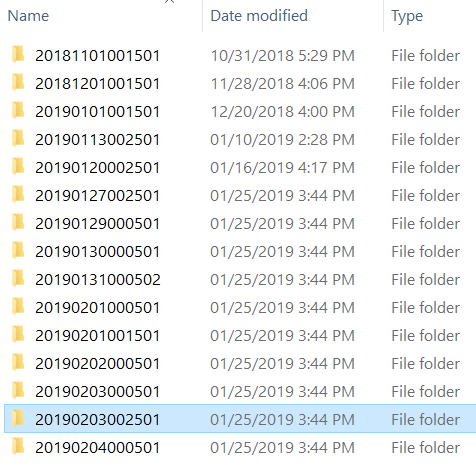 |
Each of these directories is a snapshot of the entire Scholar filesystem at the timestamp encoded into the directory name. The format for this timestamp is year, two digits for month, two digits for day, followed by the time of the day.
You may cd into any of these directories where you will find the entire Scholar filesystem. Use cd to continue into your lab's Scholar space and then you may browse the snapshot as normal.
If you are browsing these directories over a Samba network drive you can simply drag and drop the files over into your live Data Depot folder.
Once you find the file you are looking for, use cp to copy the file back into your lab's live Scholar space. Do not attempt to modify files directly in the snapshot directories.
Windows
If you use Scholar through "network drives" on Windows you may recover lost files directly from within Windows:
- Open the folder that contained the lost file.
- Right click inside the window and select "Properties".
- Click on the "Previous Versions" tab.
- A list of snapshots will be displayed.
- Select the snapshot from which you wish to restore.
- In the new window, locate the file you wish to restore.
- Simply drag the file or folder to their correct locations.
In the "Previous Versions" window the list contains two columns. The first column is the timestamp on which the snapshot was taken. The second column is the date on which the selected file or folder was last modified in that snapshot. This may give you some extra clues to which snapshot contains the version of the file you are looking for.
Mac OS X
Mac OS X does not provide any way to access the Scholar snapshots directly. To access the snapshots there are two options: browse the snapshots by hand through a network drive mount or use an automated command-line based tool.
To browse the snapshots by hand, follow the directions outlined in the Manual Browsing section.
To use the automated command-line tool, log into a compute cluster or into the host scholar.rcac.purdue.edu (which is available to all Scholar users) and use the flost tool. On Mac OS X you can use the built-in SSH terminal application to connect.
- Open the Applications folder from Finder.
- Navigate to the Utilities folder.
- Double click the Terminal application to open it.
- Type the following command when the terminal opens.
Replace myusername with your Purdue career account username and provide your password when prompted.$ ssh myusername@scholar.rcac.purdue.edu
Once logged in use the flost tool as described above. The tool will guide you through the process and show you the commands necessary to retrieve your lost file.
Gateway (Open OnDemand)
Scholar's Gateway is an open-source HPC portal developed by the Ohio Supercomputing Center. Open OnDemand allows one to interact with HPC resources through a web browser and easily manage files, submit jobs, and interact with graphical applications directly in a browser, all with no software to install. Scholar has an instance of OnDemand available that can be accessed via gateway.scholar.rcac.purdue.edu.
Link to section 'Logging In' of 'Gateway (Open OnDemand)' Logging In
To log into Gateway:
- Navigate to gateway.scholar.rcac.purdue.edu
- Log in using your Career account username and Purdue Login Duo client.
On the splash page you will see a quota usage report. If you are over 90% on any of your quotas a warning will be displayed. This information will update every 10-15 minutes while you are active on Gateway.
Link to section 'Apps' of 'Gateway (Open OnDemand)' Apps
There are a number of built-in apps in Gateway that can be accessed from the top menu bar. Below are links to documentation on each app.
Interactive Apps
There are several interactive apps available through Gateway that can be accessed through the Interactive Apps dropdown menu. These apps are provided with a basic node and software configuration as a 'quick-launch' option to get your work up and running quickly. For simplicity, minimal options are provided - these apps are not intended for complex configuration/customization scenarios.
After you a submit an interactive app to the queue, Gateway will track and manage the session. Once it starts, you may connect and disconnect from the session in your browser, leaving the job running while you log out of your browser.
Each of the available apps are documented through the following links.
Compute Node Desktop
The Compute Node Desktop app will launch a graphical desktop session on a compute node. This is similar to using Thinlinc, however, this gives you a desktop directly on a compute node instead on a front-end. This app is useful if you have a custom application or application not directly available as an interactive app you would like to run inside Gateway.
To launch a desktop session on a compute node, select the Scholar Compute Desktop app. From the submit form, select from the available options - the queue to which you wish to submit and the number of wallclock hours you wish to have job running. There is also a checkbox that enable a notification to your email when the job starts.
After the interactive job is submitted you will be taken to your list of active interactive app sessions. You can monitor the status of the job from here until it starts, or if you enabled the email notification, watch your Purdue email for the notification the job has started.
Once it is indicated the job has started you can connect to the desktop with the "Launch noVNC in New Tab" button. The session will be terminated after the wallclock hours you specified have elapsed or you terminate the session early with the "Delete" button from the list of sessions. Deleting the session when you are finished will free up queue resources for your lab mates and other users on the system.
Windows Desktop
The Windows Desktop app will launch a Windows desktop session on a compute node. This is similar to using the Windows menu launcher through Thinlinc, however, this gives you a Windows desktop directly on a compute node instead on a front-end.
To launch a Windows session on a compute node, select the Windows Desktop app. From the submit form, select from the available options - choose from the basic Windows configuration or the GIS configured image, the queue to which you wish to submit, and the number of wallclock hours you wish to have job running. There is also a checkbox that enable a notification to your email when the job starts.
This will create a file in your scratch space called windows-base.qcow2 or windows-gis.qcow2. If the file already exists, the existing image will be restarted. You can delete or rename the image at any time through the Files App to generate a fresh image. You can only have one instance of the image running at a time or corruption will occur. There are lock files to prevent this, but be mindful of this restriction. It is also recommended you make periodic backups of the image if you are making any modifications to it.
After the interactive job is submitted you will be taken to your list of active interactive app sessions. You can monitor the status of the job from here until it starts, or if you enabled the email notification, watch your Purdue email for the notification the job has started.
Once it is indicated the job has started you can connect to the desktop with the "Launch noVNC in New Tab" button. The session will be terminated after the wallclock hours you specified have elapsed or you terminate the session early with the "Delete" button from the list of sessions. Deleting the session when you are finished will free up queue resources for your lab mates and other users on the system.
Jupyter Notebook
The Notebook app will launch a Notebook session on a compute node and allow you to connect directly to it in a web browser.
To launch a Notebook session on a compute node, select the Notebook app. From the submit form, select from the available options:
- Queue: This is a dropdown menu from which you can select a queue from all of the queues to which you have permission to submit.
- Walltime: This is a field which expects a number and represents how many hours you want to keep the session running. Note that this value should not exceed the maximum value given next to the selected queue name from the queue dropdown menu.
- Number of Cores/GPUs: This is a field which expects a number and represents the number of your resources your session is requesting. Note that the amount of memory allocated for your session is proportional to the number of cores or GPUs that you request for your job, so if your session is running out of memory, consider increasing this value.
- Use Jupyter Lab: This is a checkbox which, when checked, will run Jupyter Lab instead of Jupyter Notebook. Both of these applications are interfaces to Jupyter, and you can launch Jupyter notebooks from within Jupyter Lab. Jupyter Notebook is more "barebones" while Jupyter Lab has additional features such as the ability to interact with additional file types.
- E-mail Notice: This is a checkbox which, when checked, will send you an e-mail notification to your Purdue e-mail that your session is ready when the scheduler has found resources to dedicate to your session.
After the interactive job is submitted you will be taken to your list of active interactive app sessions. You can monitor the status of the job from here until it starts, or if you enabled the email notification, watch your Purdue email for the notification the job has started.
Once it is indicated the job has started you can connect to the desktop with the "Connect to Jupyter" button. Once connected, you can create new notebooks, selecting the currently available Anaconda versions available as modules, and any personally created Notebook kernels.
Often times you may want to use one of your existing Anaconda environments within your Jupyter session to use libraries specific to your workflow. In order to do so, you must ensure that the Anaconda environment you want to use contains the Python packages "IPyKernel" and "IPython" which are packages that are required by Jupyter. When you create a Jupyter session, Open OnDemand will check through your existing Anaconda environments and create a Jupyter kernel for any Anaconda environment that contains these two packages, and you will be able to select to use that kernel from within the application.
The session will be terminated after the number of hours you specified have elapsed or you terminate the session early with the "Delete" button from the list of sessions. Deleting the session when you are finished will free up queue resources for your lab mates and other users on the system.
MATLAB
The MATLAB app will launch a MATLAB session on a compute node and allow you to connect directly to it in a web browser.
To launch a MATLAB session on a compute node, select the MATLAB app. From the submit form, select from the available options - the version of MATLAB you are interested in running, the queue to which you wish to submit, and the number of wallclock hours you wish to have job running. There is also a checkbox that enable a notification to your email when the job starts.
After the interactive job is submitted you will be taken to your list of active interactive app sessions. You can monitor the status of the job from here until it starts, or if you enabled the email notification, watch your Purdue email for the notification the job has started.
Once it is indicated the job has started you can connect to the desktop with the "Launch noVNC in New Tab" button. The session will be terminated after the wallclock hours you specified have elapsed or you terminate the session early with the "Delete" button from the list of sessions. Deleting the session when you are finished will free up queue resources for your lab mates and other users on the system.
RStudio Server
The RStudio app will launch a RStudio session on a compute node and allow you to connect directly to it in a web browser.
To launch a RStudio session on a compute node, select the RStudio app. From the submit form, select from the available options - the queue to which you wish to submit, and the number of wallclock hours you wish to have job running. There is also a checkbox that enable a notification to your email when the job starts.
After the interactive job is submitted you will be taken to your list of active interactive app sessions. You can monitor the status of the job from here until it starts, or if you enabled the email notification, watch your Purdue email for the notification the job has started.
Once it is indicated the job has started you can connect to the desktop with the "Connect to RStudio Server" button. The session will be terminated after the wallclock hours you specified have elapsed or you terminate the session early with the "Delete" button from the list of sessions. Deleting the session when you are finished will free up queue resources for your lab mates and other users on the system.
Files
The Files app will let you access your files in your Home Directory, Scratch, and Data Depot spaces. The app lets you manage create, manage, and delete files and directories from your web browser. Navigate by double clicking on folders in the file explorer or by using the file tree on the left.
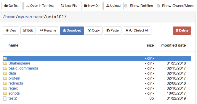
On the top row, there are buttons to:
- Go To: directly input a directory to navigate to
- Open in Terminal: launches the Shell app and navigates you to the current directory in the terminal
- New File: creates a new, empty file
- New Dir: creates a new, empty directory
- Upload: upload a file from your computer
Note: File uploads from your browser are limited to 100 GB per file. Be mindful that uploads over a few gigabytes may be unreliable through your browser, especially from off-campus connections. For very large files or off-campus transfers alternative methods such as Globus are highly recommended.
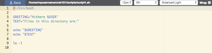
The second row of buttons lets you perform typical file management operations. The Edit button will open files in a fully fledged browser based text editor - it features syntax highlighting and vim and Emacs key bindings.
Jobs
There are two apps under the Jobs apps: Active Jobs and Job Composer. These are detailed below.
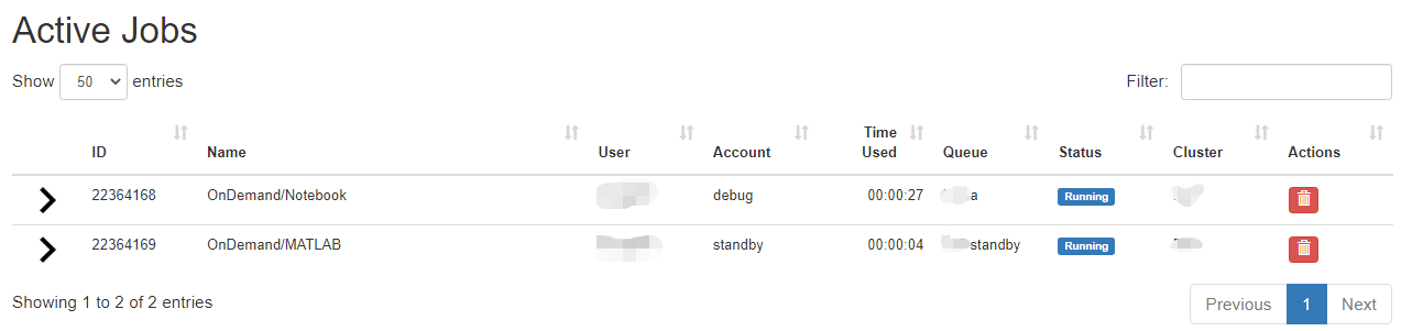
Link to section 'Active Jobs' of 'Jobs' Active Jobs
This shows you active SLURM jobs currently on the cluster. The default view will show you your current jobs, similar to squeue -u rices. Using the button labeled "Your Jobs" in the upper right allows you to select different filters by queue (account). All accounts output by slist will appear for you here. Using the arrow on the left hand side will expand the full job details.
Link to section 'Job Composer' of 'Jobs' Job Composer
The Job Composer app allows you to create and submit jobs to the cluster. You can select from pre-defined templates (most of these are taken from the User Guide examples) or you can create your own templates for frequently used workflows.
Link to section 'Creating Job from Existing Template' of 'Jobs' Creating Job from Existing Template
Click "New Job" menu, then select "From Template":
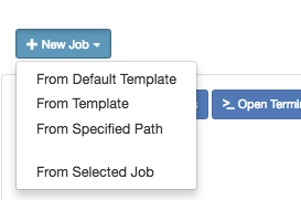
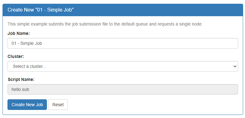
Then select from one of the available templates.
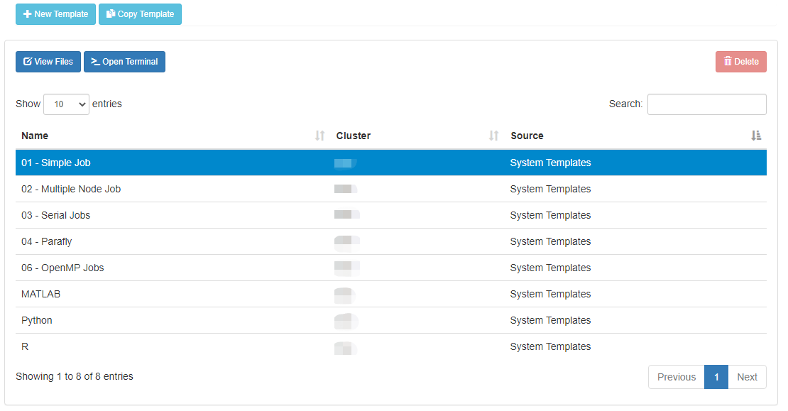
Click 'Create New Job' in second pane.
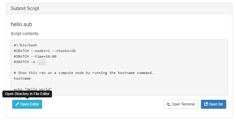
Your new job should be selected in your list of jobs. In the 'Submit Script' pane you can see the job script that was generated with an 'Open Editor' link to open the script in the built-in editor. Open the file in the editor and edit the script as necessary. By default the job will specify standby queue - this should be changed as appropriate, along with the node and walltime requests.
When you are finished with editing the job and are ready to submit, click the green 'Submit' button at the top of the job list. You can monitor progress from here or from the Active Jobs app. Once completed, you should see the output files appear:
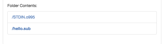
Clicking on one of the output files will open it in the file editor for your viewing.
Link to section 'Creating New Template' of 'Jobs' Creating New Template
First, prepare a template directory containing a template submission script along with any input files. Then, to import the job into the Job Composer app, click the 'Create New Template' button. Fill in the directory containing your template job script and files in the first box. Give it an appropriate name and notes.
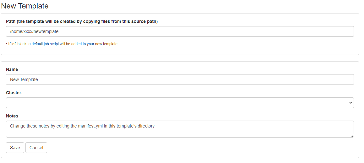
This template will now appear in your list of templates to choose from when composing jobs. You can now go create and submit a job from this new template.
Cluster Tools
The Cluster Tools menu contains cluster utilities. At the moment, only a terminal app is provided. Additional apps may be developed and provided in the future.
Link to section 'Shell Access' of 'Cluster Tools' Shell Access
Launching the shell app will provide you with a web-based terminal session on the cluster front-end. This is equivalent to using a standalone SSH client to connect to scholar.rcac.purdue.edu where you are connected to one several front-ends. The normal acceptable front-end use policy applies to access through the web-app. X11 Forwarding is not supported. Use of one of the interactive apps is recommended for graphical applications.
Software
Link to section 'Environment module' of 'Software' Environment module
Link to section 'Software catalog' of 'Software' Software catalog
Compiling Source Code
Documentation on compiling source code on Scholar.
Compiling Serial Programs
A serial program is a single process which executes as a sequential stream of instructions on one processor core. Compilers capable of serial programming are available for C, C++, and versions of Fortran.
Here are a few sample serial programs:
- serial_hello.f
- serial_hello.f90
- serial_hello.f95
- serial_hello.c
-
To load a compiler, enter one of the following:
$ module load intel
$ module load gcc
| Language | Intel Compiler | GNU Compiler | |
|---|---|---|---|
| Fortran 77 |
|
|
|
| Fortran 90 |
|
|
|
| Fortran 95 |
|
|
|
| C |
|
|
|
| C++ |
|
|
The Intel and GNU compilers will not output anything for a successful compilation. Also, the Intel compiler does not recognize the suffix ".f95".
Compiling MPI Programs
OpenMPI and Intel MPI (IMPI) are implementations of the Message-Passing Interface (MPI) standard. Libraries for these MPI implementations and compilers for C, C++, and Fortran are available on all clusters.
| Language | Header Files |
|---|---|
| Fortran 77 |
|
| Fortran 90 |
|
| Fortran 95 |
|
| C |
|
| C++ |
|
Here are a few sample programs using MPI:
To see the available MPI libraries:
$ module avail openmpi
$ module avail impi
| Language | Intel MPI | OpenMPI |
|---|---|---|
| Fortran 77 |
|
|
| Fortran 90 |
|
|
| Fortran 95 |
|
|
| C |
|
|
| C++ |
|
|
The Intel and GNU compilers will not output anything for a successful compilation. Also, the Intel compiler does not recognize the suffix ".f95".
Here is some more documentation from other sources on the MPI libraries:
Compiling OpenMP Programs
All compilers installed on Brown include OpenMP functionality for C, C++, and Fortran. An OpenMP program is a single process that takes advantage of a multi-core processor and its shared memory to achieve a form of parallel computing called multithreading. It distributes the work of a process over processor cores in a single compute node without the need for MPI communications.
| Language | Header Files |
|---|---|
| Fortran 77 |
|
| Fortran 90 |
|
| Fortran 95 |
|
| C |
|
| C++ |
|
Sample programs illustrate task parallelism of OpenMP:
A sample program illustrates loop-level (data) parallelism of OpenMP:
To load a compiler, enter one of the following:
$ module load intel
$ module load gcc
| Language | Intel Compiler | GNU Compiler |
|---|---|---|
| Fortran 77 |
|
|
| Fortran 90 |
|
|
| Fortran 95 |
|
|
| C |
|
|
| C++ |
|
|
The Intel and GNU compilers will not output anything for a successful compilation. Also, the Intel compiler does not recognize the suffix ".f95".
Here is some more documentation from other sources on OpenMP:
Compiling Hybrid Programs
A hybrid program combines both MPI and shared-memory to take advantage of compute clusters with multi-core compute nodes. Libraries for OpenMPI and Intel MPI (IMPI) and compilers which include OpenMP for C, C++, and Fortran are available.
| Language | Header Files |
|---|---|
| Fortran 77 |
|
| Fortran 90 |
|
| Fortran 95 |
|
| C |
|
| C++ |
|
A few examples illustrate hybrid programs with task parallelism of OpenMP:
This example illustrates a hybrid program with loop-level (data) parallelism of OpenMP:
To see the available MPI libraries:
$ module avail impi
$ module avail openmpi
The following tables illustrate how to compile your hybrid (MPI/OpenMP) program. Any compiler flags accepted by Intel ifort/icc compilers are compatible with their respective MPI compiler.
| Language | Command |
|---|---|
| Fortran 77 |
|
| Fortran 90 |
|
| Fortran 95 |
|
| C |
|
| C++ |
|
| Language | Command |
|---|---|
| Fortran 77 |
|
| Fortran 90 |
|
| Fortran 95 |
|
| C |
|
| C++ |
|
The Intel and GNU compilers will not output anything for a successful compilation. Also, the Intel compiler does not recognize the suffix .f95.
Intel MKL Library
Intel Math Kernel Library (MKL) contains ScaLAPACK, LAPACK, Sparse Solver, BLAS, Sparse BLAS, CBLAS, GMP, FFTs, DFTs, VSL, VML, and Interval Arithmetic routines. MKL resides in the directory stored in the environment variable MKL_HOME, after loading a version of the Intel compiler with module.
By using module load to load an Intel compiler your environment will have several variables set up to help link applications with MKL. Here are some example combinations of simplified linking options:
$ module load intel
$ echo $LINK_LAPACK
-L${MKL_HOME}/lib/intel64 -lmkl_intel_lp64 -lmkl_intel_thread -lmkl_core -liomp5 -lpthread

$ echo $LINK_LAPACK95
-L${MKL_HOME}/lib/intel64 -lmkl_lapack95_lp64 -lmkl_blas95_lp64 -lmkl_intel_lp64 -lmkl_intel_thread -lmkl_core -liomp5 -lpthread
RCAC recommends you use the provided variables to define MKL linking options in your compiling procedures. The Intel compiler modules also provide two other environment variables, LINK_LAPACK_STATIC and LINK_LAPACK95_STATIC that you may use if you need to link MKL statically.
RCAC recommends that you use dynamic linking of libguide. If so, define LD_LIBRARY_PATH such that you are using the correct version of libguide at run time. If you use static linking of libguide, then:
- If you use the Intel compilers, link in the libguide version that comes with the compiler (use the -openmp option).
- If you do not use the Intel compilers, link in the libguide version that comes with the Intel MKL above.
Here are some more documentation from other sources on the Intel MKL:
Compiling GPU Programs
The Scholar cluster nodes contain 1 GPU that support CUDA and OpenCL. See the detailed hardware overview for the specifics on the GPUs in Scholar. This section focuses on using CUDA.
A simple CUDA program has a basic workflow:
- Initialize an array on the host (CPU).
- Copy array from host memory to GPU memory.
- Apply an operation to array on GPU.
- Copy array from GPU memory to host memory.
Here is a sample CUDA program:
Both front-ends and GPU-enabled compute nodes have the CUDA tools and libraries available to compile CUDA programs. To compile a CUDA program, load CUDA, and use nvcc to compile the program:
$ module load gcc/11.4.1 cuda/12.6.0
$ nvcc gpu_hello.cu -o gpu_hello
./gpu_hello
No GPU specified, using first GPUhello, world
The example illustrates only how to copy an array between a CPU and its GPU but does not perform a serious computation.
The following program times three square matrix multiplications on a CPU and on the global and shared memory of a GPU:
$ module load cuda
$ nvcc mm.cu -o mm
$ ./mm 0
                                                            speedup
                                                            -------
Elapsed time in CPU:                    6555.2 milliseconds
Elapsed time in GPU (global memory):      32.9 milliseconds  199.1
Elapsed time in GPU (shared memory):       3.0 milliseconds  2191.8
For best performance, the input array or matrix must be sufficiently large to overcome the overhead in copying the input and output data to and from the GPU.
For more information about NVIDIA, CUDA, and GPUs:
Running Jobs
There is one method for submitting jobs to Scholar. You may use SLURM to submit jobs to a partition on Scholar. SLURM performs job scheduling. Jobs may be any type of program. You may use either the batch or interactive mode to run your jobs. Use the batch mode for finished programs; use the interactive mode only for debugging.
In this section, you'll find a few pages describing the basics of creating and submitting SLURM jobs. As well, a number of example SLURM jobs that you may be able to adapt to your own needs.
Basics of SLURM Jobs
The Simple Linux Utility for Resource Management (SLURM) is a system providing job scheduling and job management on compute clusters. With SLURM, a user requests resources and submits a job to a queue. The system will then take jobs from queues, allocate the necessary nodes, and execute them.
Do NOT run large, long, multi-threaded, parallel, or CPU-intensive jobs on a front-end login host. All users share the front-end hosts, and running anything but the smallest test job will negatively impact everyone's ability to use Scholar. Always use SLURM to submit your work as a job.
Link to section 'Submitting a Job' of 'Basics of SLURM Jobs' Submitting a Job
The main steps to submitting a job are:
Follow the links below for information on these steps, and other basic information about jobs. A number of example SLURM jobs are also available.
Queues
Link to section 'Scholar Queue' of 'Queues' Scholar Queue
This is the default queue for submitting jobs on Scholar. The maximum walltime on scholar queue is 4 hours.
Link to section 'Long Queue' of 'Queues' Long Queue
If your job requires more than 4 hours to complete, you can submit it to the long queue. The maximum walltime is 3 days. There are only 5 nodes in this queue, so you may have to wait for some time to get access to a node.
Link to section 'GPU Queue' of 'Queues' GPU Queue
If your job needs access to an Nvidia GPU accelerator, then use the gpu queue. The maximum walltime is 4 hours.
Link to section 'Debug Queue' of 'Queues' Debug Queue
The debug queue allows you to quickly start small, short, interactive jobs in order to debug code, test programs, or test configurations. You are limited to one running job at a time in the queue, and you may run up to two compute nodes for 30 minutes. The expectation is that debug jobs should start within a couple of minutes, assuming all of its dedicated nodes are not taken by others.
Link to section 'List of Queues' of 'Queues' List of Queues
To see a list of all queues on Scholar that you may submit to, use the slist command
This lists each queue you can submit to, the number of nodes allocated to the queue, how many are available to run jobs, and the maximum walltime you may request. Options to the command will give more detailed information. This command can be used to get a general idea of how busy an individual queue is and how long you may have to wait for your job to start.
Job Submission Script
To submit work to a SLURM queue, you must first create a job submission file. This job submission file is essentially a simple shell script. It will set any required environment variables, load any necessary modules, create or modify files and directories, and run any applications that you need:
#!/bin/bash
# FILENAME:  myjobsubmissionfile

# Loads Matlab and sets the application up
module load matlab

# Change to the directory from which you originally submitted this job.
cd $SLURM_SUBMIT_DIR

# Runs a Matlab script named 'myscript'
matlab -nodisplay -singleCompThread -r myscript
Once your script is prepared, you are ready to submit your job.
Link to section 'Job Script Environment Variables' of 'Job Submission Script' Job Script Environment Variables
| Name | Description |
|---|---|
| SLURM_SUBMIT_DIR | Absolute path of the current working directory when you submitted this job |
| SLURM_JOBID | Job ID number assigned to this job by the batch system |
| SLURM_JOB_NAME | Job name supplied by the user |
| SLURM_JOB_NODELIST | Names of nodes assigned to this job |
| SLURM_CLUSTER_NAME | Name of the cluster executing the job |
| SLURM_SUBMIT_HOST | Hostname of the system where you submitted this job |
| SLURM_JOB_PARTITION | Name of the original queue to which you submitted this job |
Submitting a Job
Once you have a job submission file, you may submit this script to SLURM using the sbatch command. SLURM will find, or wait for, available resources matching your request and run your job there.
To submit your job to one compute node:
$ sbatch --nodes=1 myjobsubmissionfile
Slurm uses the word 'Account' and the option '-A' to specify different batch queues. To submit your job to a specific queue:
$ sbatch --nodes=1 -A scholar myjobsubmissionfile
By default, each job receives 30 minutes of wall time, or clock time. If you know that your job will not need more than a certain amount of time to run, request less than the maximum wall time, as this may allow your job to run sooner. To request the 1 hour and 30 minutes of wall time:
$ sbatch -t 1:30:00 --nodes=1 -A scholar myjobsubmissionfile
The --nodes value indicates how many compute nodes you would like for your job.
Each compute node in Scholar has 20 processor cores.
In some cases, you may want to request multiple nodes. To utilize multiple nodes, you will need to have a program or code that is specifically programmed to use multiple nodes such as with MPI. Simply requesting more nodes will not make your work go faster. Your code must support this ability.
To request 2 compute nodes:
$ sbatch --nodes=2 myjobsubmissionfile
By default, jobs on Scholar will share nodes with other jobs.
To submit a job using 1 compute node with 4 tasks, each using the default 1 core and 1 GPU per node:
$ sbatch --nodes=1 --ntasks=4 --gpus-per-node=1 myjobsubmissionfile
If more convenient, you may also specify any command line options to sbatch from within your job submission file, using a special form of comment:
#!/bin/sh -l
# FILENAME:  myjobsubmissionfile

#SBATCH -A myqueuename
#SBATCH --nodes=1
#SBATCH --time=1:30:00
#SBATCH --job-name myjobname

# Print the hostname of the compute node on which this job is running.
/bin/hostname
If an option is present in both your job submission file and on the command line, the option on the command line will take precedence.
After you submit your job with SBATCH, it may wait in queue for minutes, hours, or even weeks. How long it takes for a job to start depends on the specific queue, the resources and time requested, and other jobs already waiting in that queue requested as well. It is impossible to say for sure when any given job will start. For best results, request no more resources than your job requires.
Once your job is submitted, you can monitor the job status, wait for the job to complete, and check the job output.
Job Dependencies
Dependencies are an automated way of holding and releasing jobs. Jobs with a dependency are held until the condition is satisfied. Once the condition is satisfied jobs only then become eligible to run and must still queue as normal.
Job dependencies may be configured to ensure jobs start in a specified order. Jobs can be configured to run after other job state changes, such as when the job starts or the job ends.
These examples illustrate setting dependencies in several ways. Typically dependencies are set by capturing and using the job ID from the last job submitted.
To run a job after job myjobid has started:
sbatch --dependency=after:myjobid myjobsubmissionfile
To run a job after job myjobid ends without error:
sbatch --dependency=afterok:myjobid myjobsubmissionfile
To run a job after job myjobid ends with errors:
sbatch --dependency=afternotok:myjobid myjobsubmissionfile
To run a job after job myjobid ends with or without errors:
sbatch --dependency=afterany:myjobid myjobsubmissionfile
To set more complex dependencies on multiple jobs and conditions:
sbatch --dependency=after:myjobid1:myjobid2:myjobid3,afterok:myjobid4 myjobsubmissionfile
Holding a Job
Sometimes you may want to submit a job but not have it run just yet. You may be wanting to allow lab mates to cut in front of you in the queue - so hold the job until their jobs have started, and then release yours.
To place a hold on a job before it starts running, use the scontrol hold job command:
$ scontrol hold job myjobid
Once a job has started running it can not be placed on hold.
To release a hold on a job, use the scontrol release job command:
$ scontrol release job myjobid
You find the job ID using the squeue command as explained in the SLURM Job Status section.
Checking Job Status
Once a job is submitted there are several commands you can use to monitor the progress of the job.
To see your jobs, use the squeue -u command and specify your username:
(Remember, in our SLURM environment a queue is referred to as an 'Account')
squeue -u myusername

    JOBID   ACCOUNT    NAME    USER   ST    TIME   NODES  NODELIST(REASON)
   182792   scholar    job1    myusername    R   20:19       1  scholar-a000
   185841   scholar    job2    myusername    R   20:19       1  scholar-a001
   185844   scholar    job3    myusername    R   20:18       1  scholar-a002
   185847   scholar    job4    myusername    R   20:18       1  scholar-a003
To retrieve useful information about your queued or running job, use the scontrol show job command with your job's ID number. The output should look similar to the following:
scontrol show job 3519

JobId=3519 JobName=t.sub
   UserId=myusername GroupId=mygroup MCS_label=N/A
   Priority=3 Nice=0 Account=(null) QOS=(null)
   JobState=PENDING Reason=BeginTime Dependency=(null)
   Requeue=1 Restarts=0 BatchFlag=1 Reboot=0 ExitCode=0:0
   RunTime=00:00:00 TimeLimit=7-00:00:00 TimeMin=N/A
   SubmitTime=2019-08-29T16:56:52 EligibleTime=2019-08-29T23:30:00
   AccrueTime=Unknown
   StartTime=2019-08-29T23:30:00 EndTime=2019-09-05T23:30:00 Deadline=N/A
   PreemptTime=None SuspendTime=None SecsPreSuspend=0
   LastSchedEval=2019-08-29T16:56:52
   Partition=workq AllocNode:Sid=mack-fe00:54476
   ReqNodeList=(null) ExcNodeList=(null)
   NodeList=(null)
   NumNodes=1 NumCPUs=2 NumTasks=2 CPUs/Task=1 ReqB:S:C:T=0:0:*:*
   TRES=cpu=2,node=1,billing=2
   Socks/Node=* NtasksPerN:B:S:C=0:0:*:* CoreSpec=*
   MinCPUsNode=1 MinMemoryNode=0 MinTmpDiskNode=0
   Features=(null) DelayBoot=00:00:00
   OverSubscribe=OK Contiguous=0 Licenses=(null) Network=(null)
   Command=/home/myusername/jobdir/myjobfile.sub
   WorkDir=/home/myusername/jobdir
   StdErr=/home/myusername/jobdir/slurm-3519.out
   StdIn=/dev/null
   StdOut=/home/myusername/jobdir/slurm-3519.out
   Power=
There are several useful bits of information in this output.
JobStatelets you know if the job is Pending, Running, Completed, or Held.RunTime and TimeLimitwill show how long the job has run and its maximum time.SubmitTimeis when the job was submitted to the cluster.NumNodes,NumCPUs,NumTasksandCPUs/Taskare the number of Nodes, CPUs, Tasks, and CPUs per Task are shown.WorkDiris the job's working directory.StdOutandStderrare the locations of stdout and stderr of the job, respectively.Reasonwill show why aPENDINGjob isn't running. The above error says that it has been requested to start at a specific, later time.
Checking Job Output
Once a job is submitted, and has started, it will write its standard output and standard error to files that you can read.
SLURM catches output written to standard output and standard error - what would be printed to your screen if you ran your program interactively. Unless you specfied otherwise, SLURM will put the output in the directory where you submitted the job in a file named slurm- followed by the job id, with the extension out. For example slurm-3509.out. Note that both stdout and stderr will be written into the same file, unless you specify otherwise.
If your program writes its own output files, those files will be created as defined by the program. This may be in the directory where the program was run, or may be defined in a configuration or input file. You will need to check the documentation for your program for more details.
Link to section 'Redirecting Job Output' of 'Checking Job Output' Redirecting Job Output
It is possible to redirect job output to somewhere other than the default location with the --error and --output directives:
#!/bin/bash
#SBATCH --output=/home/myusername/joboutput/myjob.out
#SBATCH --error=/home/myusername/joboutput/myjob.out

# This job prints "Hello World" to output and exits
echo "Hello World"
Canceling a Job
To stop a job before it finishes or remove it from a queue, use the scancel command:
scancel myjobid
You find the job ID using the squeue command as explained in the SLURM Job Status section.
Example Jobs
A number of example jobs are available for you to look over and adapt to your own needs. The first few are generic examples, and latter ones go into specifics for particular software packages.
Generic SLURM Jobs
The following examples demonstrate the basics of SLURM jobs, and are designed to cover common job request scenarios. These example jobs will need to be modified to run your application or code.
Simple Job
Every SLURM job consists of a job submission file. A job submission file contains a list of commands that run your program and a set of resource (nodes, walltime, queue) requests. The resource requests can appear in the job submission file or can be specified at submit-time as shown below.
This simple example submits the job submission file hello.sub to the scholar queue on Scholar and requests a single node:
#!/bin/bash
# FILENAME: hello.sub

# Show this ran on a compute node by running the hostname command.
hostname

echo "Hello World"
sbatch -A scholar --nodes=1 --ntasks=1 --cpus-per-task=1 --time=00:01:00 hello.sub
Submitted batch job 3521
For a real job you would replace echo "Hello World" with a command, or sequence of commands, that run your program.
After your job finishes running, the ls command will show a new file in your directory, the .out file:
ls -l
hello.sub
slurm-3521.out
The file slurm-3521.out contains the output and errors your program would have written to the screen if you had typed its commands at a command prompt:
cat slurm-3521.out


scholar-a001.rcac.purdue.edu
Hello World
You should see the hostname of the compute node your job was executed on. Following should be the "Hello World" statement.
Multiple Node
In some cases, you may want to request multiple nodes. To utilize multiple nodes, you will need to have a program or code that is specifically programmed to use multiple nodes such as with MPI. Simply requesting more nodes will not make your work go faster. Your code must support this ability.
This example shows a request for multiple compute nodes. The job submission file contains a single command to show the names of the compute nodes allocated:
# FILENAME:  myjobsubmissionfile.sub
#!/bin/bash
echo "$SLURM_JOB_NODELIST"
sbatch --nodes=2 --ntasks=40 --time=00:10:00 -A scholar myjobsubmissionfile.sub
Compute nodes allocated:
scholar-a[014-015]
The above example will allocate the total of 40 CPU cores across 2 nodes. Note that if your multi-node job requests fewer than each node's full 20 cores per node, by default Slurm provides no guarantee with respect to how this total is distributed between assigned nodes (i.e. the cores may not necessarily be split evenly). If you need specific arrangements of your tasks and cores, you can use --cpus-per-task= and/or --ntasks-per-node= flags. See Slurm documentation or man sbatch for more options.
Directives
So far these examples have shown submitting jobs with the resource requests on the sbatch command line such as:
sbatch -A scholar --nodes=1 --time=00:01:00 hello.sub
The resource requests can also be put into job submission file itself. Documenting the resource requests in the job submission is desirable because the job can be easily reproduced later. Details left in your command history are quickly lost. Arguments are specified with the #SBATCH syntax:
#!/bin/bash

# FILENAME: hello.sub

#SBATCH -A scholar

#SBATCH --nodes=1 --time=00:01:00

# Show this ran on a compute node by running the hostname command.
hostname

echo "Hello World"
The #SBATCH directives must appear at the top of your submission file. SLURM will stop parsing directives as soon as it encounters a line that does not start with '#'. If you insert a directive in the middle of your script, it will be ignored.
This job can be then submitted with:
sbatch hello.sub
Specific Types of Nodes
SLURM allows running a job on specific types of compute nodes to accommodate special hardware requirements (e.g. a certain CPU or GPU type, etc.)
Cluster nodes have a set of descriptive features assigned to them, and users can specify which of these features are required by their job by using the constraint option at submission time. Only nodes having features matching the job constraints will be used to satisfy the request.
Example: a job requires a compute node in an "A" sub-cluster:
sbatch --nodes=1 --ntasks=20 --constraint=A myjobsubmissionfile.subCompute node allocated:
scholar-a003Feature constraints can be used for both batch and interactive jobs, as well as for individual job steps inside a job. Multiple constraints can be specified with a predefined syntax to achieve complex request logic (see detailed description of the '--constraint' option in man sbatch or online Slurm documentation).
Refer to Detailed Hardware Specification section for list of available sub-cluster labels, their respective per-node memory sizes and other hardware details. You could also use sfeatures command to list available constraint feature names for different node types.
Interactive Jobs
Interactive jobs are run on compute nodes, while giving you a shell to interact with. They give you the ability to type commands or use a graphical interface in the same way as if you were on a front-end login host.
To submit an interactive job, use sinteractive to run a login shell on allocated resources.
sinteractive accepts most of the same resource requests as sbatch, so to request a login shell on the cpu account while allocating 2 nodes and 20 total cores, you might do:
sinteractive -A cpu -N2 -n40
To quit your interactive job:
exit or Ctrl-D
The above example will allocate the total of 40 CPU cores across 2 nodes. Note that if your multi-node job requests fewer than each node's full 20 cores per node, by default Slurm provides no guarantee with respect to how this total is distributed between assigned nodes (i.e. the cores may not necessarily be split evenly). If you need specific arrangements of your tasks and cores, you can use --cpus-per-task= and/or --ntasks-per-node= flags. See Slurm documentation or man salloc for more options.
Serial Jobs
This shows how to submit one of the serial programs compiled in the section Compiling Serial Programs.
Create a job submission file:
#!/bin/bash
# FILENAME:  serial_hello.sub

./serial_hello
Submit the job:
sbatch --nodes=1 --ntasks=1 --time=00:01:00 serial_hello.sub
After the job completes, view results in the output file:
cat slurm-myjobid.out

Runhost:scholar-a009.rcac.purdue.edu
hello, world
If the job failed to run, then view error messages in the file slurm-myjobid.out.
OpenMP
A shared-memory job is a single process that takes advantage of a multi-core processor and its shared memory to achieve parallelization.
This example shows how to submit an OpenMP program compiled in the section Compiling OpenMP Programs.
When running OpenMP programs, all threads must be on the same compute node to take advantage of shared memory. The threads cannot communicate between nodes.
To run an OpenMP program, set the environment variable OMP_NUM_THREADS to the desired number of threads:
In csh:
setenv OMP_NUM_THREADS 20In bash:
export OMP_NUM_THREADS=20This should almost always be equal to the number of cores on a compute node. You may want to set to another appropriate value if you are running several processes in parallel in a single job or node.
Create a job submissionfile:
#!/bin/bash
# FILENAME:  omp_hello.sub
#SBATCH --nodes=1
#SBATCH --ntasks=20
#SBATCH --time=00:01:00

export OMP_NUM_THREADS=20
./omp_hello
Submit the job:
sbatch omp_hello.subView the results from one of the sample OpenMP programs about task parallelism:
cat omp_hello.sub.omyjobid
SERIAL REGION:     Runhost:scholar-a003.rcac.purdue.edu   Thread:0 of 1 thread    hello, world
PARALLEL REGION:   Runhost:scholar-a003.rcac.purdue.edu   Thread:0 of 20 threads   hello, world
PARALLEL REGION:   Runhost:scholar-a003.rcac.purdue.edu   Thread:1 of 20 threads   hello, world
   ...
If the job failed to run, then view error messages in the file slurm-myjobid.out.
If an OpenMP program uses a lot of memory and 20 threads use all of the memory of the compute node, use fewer processor cores (OpenMP threads) on that compute node.
MPI
An MPI job is a set of processes that take advantage of multiple compute nodes by communicating with each other. OpenMPI and Intel MPI (IMPI) are implementations of the MPI standard.
This section shows how to submit one of the MPI programs compiled in the section Compiling MPI Programs.
Use module load to set up the paths to access these libraries. Use module avail to see all MPI packages installed on Scholar.
Create a job submission file:
#!/bin/bash
# FILENAME:  mpi_hello.sub
#SBATCH  --nodes=2
#SBATCH  --ntasks-per-node=20
#SBATCH  --time=00:01:00
#SBATCH  -A scholar

srun -n 40 ./mpi_hello
SLURM can run an MPI program with the srun command. The number of processes is requested with the -n option. If you do not specify the -n option, it will default to the total number of processor cores you request from SLURM.
If the code is built with OpenMPI, it can be run with a simple srun -n command. If it is built with Intel IMPI, then you also need to add the --mpi=pmi2 option: srun --mpi=pmi2 -n 40 ./mpi_hello in this example.
Submit the MPI job:
sbatch ./mpi_hello.subView results in the output file:
cat slurm-myjobid.out
Runhost:scholar-a010.rcac.purdue.edu   Rank:0 of 40 ranks   hello, world
Runhost:scholar-a010.rcac.purdue.edu   Rank:1 of 40 ranks   hello, world
...
Runhost:scholar-a011.rcac.purdue.edu   Rank:20 of 40 ranks   hello, world
Runhost:scholar-a011.rcac.purdue.edu   Rank:21 of 40 ranks   hello, world
...
If the job failed to run, then view error messages in the output file.
If an MPI job uses a lot of memory and 20 MPI ranks per compute node use all of the memory of the compute nodes, request more compute nodes, while keeping the total number of MPI ranks unchanged.
Submit the job with double the number of compute nodes and modify the resource request to halve the number of MPI ranks per compute node.
#!/bin/bash
# FILENAME:  mpi_hello.sub

#SBATCH --nodes=4
#SBATCH --ntasks-per-node=10
#SBATCH -t 00:01:00
#SBATCH -A scholar

srun -n 40 ./mpi_hello
sbatch ./mpi_hello.subView results in the output file:
cat slurm-myjobid.out
Runhost:scholar-a10.rcac.purdue.edu   Rank:0 of 40 ranks   hello, world
Runhost:scholar-a010.rcac.purdue.edu   Rank:1 of 40 ranks   hello, world
...
Runhost:scholar-a011.rcac.purdue.edu   Rank:10 of 40 ranks   hello, world
...
Runhost:scholar-a012.rcac.purdue.edu   Rank:20 of 40 ranks   hello, world
...
Runhost:scholar-a013.rcac.purdue.edu   Rank:30 of 40 ranks   hello, world
...
Notes
- Use slist to determine which queues (
--accountor-Aoption) are available to you. The name of the queue which is available to everyone on Scholar is "scholar". - Invoking an MPI program on Scholar with ./program is typically wrong, since this will use only one MPI process and defeat the purpose of using MPI. Unless that is what you want (rarely the case), you should use srun or mpiexec to invoke an MPI program.
- In general, the exact order in which MPI ranks output similar write requests to an output file is random.
GPU
The Scholar cluster nodes contain NVIDIA GPUs that support CUDA and OpenCL. See the detailed hardware overview for the specifics on the GPUs in Scholar.
This section illustrates how to use SLURM to submit a simple GPU program.
Suppose that you named your executable file gpu_hello from the sample code gpu_hello.cu (see the section on compiling NVIDIA GPU codes). Prepare a job submission file with an appropriate name, here named gpu_hello.sub:
#!/bin/bash
# FILENAME:  gpu_hello.sub

module load cuda

host=`hostname -s`

echo $CUDA_VISIBLE_DEVICES

# Run on the first available GPU
./gpu_hello 0
Submit the job:
sbatch -A gpu --nodes=1 --gres=gpu:1 -t 00:01:00 gpu_hello.sub
Requesting a GPU from the scheduler is required.
You can specify total number of GPUs, or number of GPUs per node, or even number of GPUs per task:
sbatch -A gpu --nodes=1 --gres=gpu:1 -t 00:01:00 gpu_hello.sub
sbatch -A gpu --nodes=1 --gpus-per-node=1 -t 00:01:00 gpu_hello.sub
sbatch -A gpu --nodes=1 --gpus-per-task=1 -t 00:01:00 gpu_hello.sub
After job completion, view the new output file in your directory:
ls -l
gpu_hello
gpu_hello.cu
gpu_hello.sub
slurm-myjobid.out
View results in the file for all standard output, slurm-myjobid.out
0
hello, world
If the job failed to run, then view error messages in the file slurm-myjobid.out.
To use multiple GPUs in your job, simply specify a larger value to the GPU specification parameter. However, be aware of the number of GPUs installed on the node(s) you may be requesting. The scheduler can not allocate more GPUs than physically exist. See detailed hardware overview and output of sfeatures command for the specifics on the GPUs in Scholar.
Link to section 'Collecting System Resource Utilization Data' of 'Monitoring Resources' Collecting System Resource Utilization Data
Knowing the precise resource utilization an application had during a job, such as CPU load or memory, can be incredibly useful. This is especially the case when the application isn't performing as expected.
One approach is to run a program like htop during an interactive job and keep an eye on system resources. You can get precise time-series data from nodes associated with your job using XDmod as well, online. But these methods don't gather telemetry in an automated fashion, nor do they give you control over the resolution or format of the data.
As a matter of course, a robust implementation of some HPC workload would include resource utilization data as a diagnostic tool in the event of some failure.
The monitor utility is a simple command line system resource monitoring tool for gathering such telemetry and is available as a module.
module load monitor
Complete documentation is available online at resource-monitor.readthedocs.io. A full manual page is also available for reference, man monitor.
In the context of a SLURM job you will need to put this monitoring task in the background to allow the rest of your job script to proceed. Be sure to interrupt these tasks at the end of your job.
#!/bin/bash
# FILENAME: monitored_job.sh

 module load monitor

# track per-code CPU load
monitor cpu percent --all-cores >cpu-percent.log &
CPU_PID=$!

# track memory usage
monitor cpu memory >cpu-memory.log &
MEM_PID=$!

# your code here

# shut down the resource monitors
kill -s INT $CPU_PID $MEM_PID
A particularly elegant solution would be to include such tools in your prologue script and have the tear down in your epilogue script.
For large distributed jobs spread across multiple nodes, mpiexec can be used to gather telemetry from all nodes in the job. The hostname is included in each line of output so that data can be grouped as such. A concise way of constructing the needed list of hostnames in SLURM is to simply use srun hostname | sort -u.
#!/bin/bash
# FILENAME: monitored_job.sh

module load monitor

# track all CPUs (one monitor per host)
mpiexec -machinefile <(srun hostname | sort -u) \
    monitor cpu percent --all-cores >cpu-percent.log &
CPU_PID=$!

# track memory on all hosts (one monitor per host)
mpiexec -machinefile <(srun hostname | sort -u) \
    monitor cpu memory >cpu-memory.log &
MEM_PID=$!

# your code here

# shut down the resource monitors
kill -s INT $CPU_PID $MEM_PID
To get resource data in a more readily computable format, the monitor program can be told to output in CSV format with the --csv flag.
monitor cpu memory --csv >cpu-memory.csv
For a distributed job you will need to suppress the header lines otherwise one will be created by each host.
monitor cpu memory --csv | head -1 >cpu-memory.csv
mpiexec -machinefile <(srun hostname | sort -u) \
    monitor cpu memory --csv --no-header >>cpu-memory.csv
Specific Applications
The following examples demonstrate job submission files for some common real-world applications. See the Generic SLURM Examples section for more examples on job submissions that can be adapted for use.
Gaussian
Gaussian is a computational chemistry software package which works on electronic structure. This section illustrates how to submit a small Gaussian job to a Slurm queue. This Gaussian example runs the Fletcher-Powell multivariable optimization.
Prepare a Gaussian input file with an appropriate filename, here named myjob.com. The final blank line is necessary:
#P TEST OPT=FP STO-3G OPTCYC=2

STO-3G FLETCHER-POWELL OPTIMIZATION OF WATER

0 1
O
H 1 R
H 1 R 2 A

R 0.96
A 104.
To submit this job, load Gaussian then run the provided script, named subg16. This job uses one compute node with 20 processor cores:
module load gaussian16
subg16 myjob -N 1 -n 20
View job status:
squeue -u myusername
View results in the file for Gaussian output, here named myjob.log. Only the first and last few lines appear here:
 Entering Gaussian System, Link 0=/apps/cent7/gaussian/g16-A.03/g16-haswell/g16/g16
 Initial command:

 /apps/cent7/gaussian/g16-A.03/g16-haswell/g16/l1.exe /scratch/scholar/myusername/gaussian/Gau-7781.inp -scrdir=/scratch/scholar/myusername/gaussian/
 Entering Link 1 = /apps/cent7/gaussian/g16-A.03/g16-haswell/g16/l1.exe PID=      7782.

 Copyright (c) 1988,1990,1992,1993,1995,1998,2003,2009,2016,
            Gaussian, Inc.  All Rights Reserved.

.
.
.

 Job cpu time:       0 days  0 hours  3 minutes 28.2 seconds.
 Elapsed time:       0 days  0 hours  0 minutes 12.9 seconds.
 File lengths (MBytes):  RWF=     17 Int=      0 D2E=      0 Chk=      2 Scr=      2
 Normal termination of Gaussian 16 at Tue May  1 17:12:00 2018.
real 13.85
user 202.05
sys 6.12
Machine:
scholar-a012.rcac.purdue.edu
scholar-a012.rcac.purdue.edu
scholar-a012.rcac.purdue.edu
scholar-a012.rcac.purdue.edu
scholar-a012.rcac.purdue.edu
scholar-a012.rcac.purdue.edu
scholar-a012.rcac.purdue.edu
scholar-a012.rcac.purdue.edu
Link to section 'Examples of Gaussian SLURM Job Submissions' of 'Gaussian' Examples of Gaussian SLURM Job Submissions
Submit job using 20 processor cores on a single node:
subg16 myjob -N 1 -n 20 -t 200:00:00 -A myqueuename
Submit job using 20 processor cores on each of 2 nodes:
subg16 myjob -N 2 --ntasks-per-node=20 -t 200:00:00 -A myqueuename
To submit a bash job, a submit script sample looks like:
#!/bin/bash

#SBATCH -A myqueuename  # Queue name(use 'slist' command to find queues' name)
#SBATCH --nodes=1       # Total # of nodes
#SBATCH --ntasks=64     # Total # of MPI tasks
#SBATCH --time=1:00:00  # Total run time limit (hh:mm:ss)
#SBATCH -J myjobname    # Job name
#SBATCH -o myjob.o%j    # Name of stdout output file
#SBATCH -e myjob.e%j    # Name of stderr error file

module load gaussian16

g16 < myjob.com
For more information about Gaussian:
Machine Learning
Machine Learning packages are now best installed through conda, which has available repositories for all major machine learning frameworks. conda can be loaded via module load conda.
ML-Toolkit
A set of pre-installed popular machine learning (ML) libraries, called ML-Toolkit is maintained on Scholar. These are Anaconda/Python-based distributions of the respective libraries. Currently, applications are supported for Python 2 and 3. Detailed instructions for searching and using the installed ML applications are presented below.
Link to section 'Instructions for using ML-Toolkit Modules' of 'ML-Toolkit' Instructions for using ML-Toolkit Modules
Link to section 'Find and Use Installed ML Packages' of 'ML-Toolkit' Find and Use Installed ML Packages
To search or load a machine learning application, you must first load one of the learning modules. The learning module loads the prerequisites (such as anaconda and cudnn) and makes ML applications visible to the user.
Step 1. Find and load a preferred learning module. Several learning modules may be available, corresponding to a specific Python version and whether the ML applications have GPU support or not. Running module load learning without specifying a version will load the version with the most recent python version. To see all available modules, run module spider learning then load the desired module.
Step 2. Find and load the desired machine learning libraries
ML packages are installed under the common application name ml-toolkit-X, where X can be cpu or gpu.
You can use the module spider ml-toolkit command to see all options and versions of each library.
Load the desired modules using the module load command. Note that both CPU and GPU options may exist for many libraries, so be sure to load the correct version. For example, if you wanted to load the most recent version of PyTorch for CPU, you would run module load ml-toolkit-cpu/pytorch
caffe          cntk          gym          keras          mxnet
opencv         pytorch       tensorflow   tflearn        theano
Step 3. You can list which ML applications are loaded in your environment using the command module list
Link to section 'Verify application import' of 'ML-Toolkit' Verify application import
Step 4. The next step is to check that you can actually use the desired ML application. You can do this by running the import command in Python. The example below tests if PyTorch has been loaded correctly.
python -c "import torch; print(torch.__version__)"
If the import operation succeeded, then you can run your own ML code. Some ML applications (such as tensorflow) print diagnostic warnings while loading -- this is the expected behavior.
If the import fails with an error, please see the troubleshooting information below.
Step 5. To load a different set of applications, unload the previously loaded applications and load the new desired applications. The example below loads Tensorflow and Keras instead of PyTorch and OpenCV.
module unload ml-toolkit-cpu/opencv
module unload ml-toolkit-cpu/pytorch
module load ml-toolkit-cpu/tensorflow
module load ml-toolkit-cpu/keras
Link to section 'Troubleshooting' of 'ML-Toolkit' Troubleshooting
ML applications depend on a wide range of Python packages and mixing multiple versions of these packages can lead to error. The following guidelines will assist you in identifying the cause of the problem.
- Check that you are using the correct version of Python with the command python --version. This should match the Python version in the loaded anaconda module.
- Start from a clean environment. Either start a new terminal session or unload all the modules using module purge. Then load the desired modules following Steps 1-2.
- Verify that PYTHONPATH does not point to undesired packages. Run the following command to print PYTHONPATH: echo $PYTHONPATH. Make sure that your Python environment is clean. Watch out for any locally installed packages that might conflict.
- If you don't see GPU devices in your code, make sure that you are using the ml-toolkit-gpu/ modules and not using their cpu versions.
- ML applications often have dependency on specific versions of Cuda and CuDNN libraries. Make sure that you have loaded the required versions using the command: module list
- Note that Caffe has a conflicting version of PyQt5. So, if you want to use Spyder (or any GUI application that uses PyQt), then you should unload the caffe module.
- Use Google search to your advantage. Copy the error message in Google and check probable causes.
More examples showing how to use ml-toolkit modules in a batch job are presented in ML Batch Jobs guide.
Link to section 'Installation of Custom ML Libraries' of 'Custom ML Packages' Installation of Custom ML Libraries
While we try to include as many common ML frameworks and versions as we can in ML-Toolkit, we recognize that there are also situations in which a custom installation may be preferable. We recommend using conda-env-mod to install and manage Python packages. Please follow the steps carefully, otherwise you may end up with a faulty installation. The example below shows how to install TensorFlow in your home directory.
Link to section 'Install' of 'Custom ML Packages' Install
Step 1: Unload all modules and start with a clean environment.
module purge
Step 2: Load the anaconda module with desired Python version.
module load anaconda
Step 2A: If the ML application requires Cuda and CuDNN, load the appropriate modules. Be sure to check that the versions you load are compatible with the desired ML package.
module load cuda
module load cudnn
Many machine-learning packages (including PyTorch and TensorFlow) now provide installation pathways that include the full cudatoolkit within the environment, making it unnecessary to load these modules.
Step 3: Create a custom anaconda environment. Make sure the python version matches the Python version in the anaconda module.
conda-env-mod create -n env_name_here
Step 4: Activate the anaconda environment by loading the modules displayed at the end of step 3.
module load use.own
module load conda-env/env_name_here-py3.6.4
Step 5: Now install the desired ML application. You can install multiple Python packages at this step using either conda or pip.
pip install --ignore-installed tensorflow==2.6
If the installation succeeded, you can now proceed to testing and using the installed application. You must load the environment you created as well as any supporting modules (e.g., anaconda) whenever you want to use this installation. If your installation did not succeed, please refer to the troubleshooting section below as well as documentation for the desired package you are installing.
Note that loading the modules generated by conda-env-mod has different behavior than conda create env_name_here followed by source activate env_name_here. After running source activate, you may not be able to access any Python packages in anaconda or ml-toolkit modules. Therefore, using conda-env-mod is the preferred way of using your custom installations.
Link to section 'Testing the Installation' of 'Custom ML Packages' Testing the Installation
-
Verify the installation by using a simple import statement, like that listed below for TensorFlow:
python -c "import tensorflow as tf; print(tf.__version__);"Note that a successful import of TensorFlow will print a variety of system and hardware information. This is expected.
If importing the package leads to errors, be sure to verify that all dependencies for the package have been managed, and the correct versions installed. Dependency issues between python packages are the most common cause for errors. For example, in TF, conflicts with the h5py or numpy versions are common, but upgrading those packages typically solves the problem. Managing dependencies for ML libraries can be non-trivial.
-
Next, we can test using our installation of TensorFlow for a GPU run. For this we shall use the matrix multiplication example from Tensorflow documentation.
# filename: matrixmult.py import tensorflow as tf print("Num GPUs Available: ", len(tf.config.list_physical_devices('GPU'))) tf.debugging.set_log_device_placement(True) # Place tensors on the CPU with tf.device('/CPU:0'): a = tf.constant([[1.0, 2.0, 3.0], [4.0, 5.0, 6.0]]) b = tf.constant([[1.0, 2.0], [3.0, 4.0], [5.0, 6.0]]) # Run on the GPU c = tf.matmul(a, b) print(c) -
Run the example
$ python matrixmult.py -
This will produce an output like:
Num GPUs Available: 3 2022-07-25 10:33:23.358919: I tensorflow/core/platform/cpu_feature_guard.cc:193] This TensorFlow binary is optimized with oneAPI Deep Neural Network Library (oneDNN) to use the following CPU instructions in performance-critical operations: AVX2 AVX512F FMA To enable them in other operations, rebuild TensorFlow with the appropriate compiler flags. 2022-07-25 10:33:26.223459: I tensorflow/core/common_runtime/gpu/gpu_device.cc:1532] Created device /job:localhost/replica:0/task:0/device:GPU:0 with 22183 MB memory: -> device: 0, name: NVIDIA A30, pci bus id: 0000:3b:00.0, compute capability: 8.0 2022-07-25 10:33:26.225495: I tensorflow/core/common_runtime/gpu/gpu_device.cc:1532] Created device /job:localhost/replica:0/task:0/device:GPU:1 with 22183 MB memory: -> device: 1, name: NVIDIA A30, pci bus id: 0000:af:00.0, compute capability: 8.0 2022-07-25 10:33:26.228514: I tensorflow/core/common_runtime/gpu/gpu_device.cc:1532] Created device /job:localhost/replica:0/task:0/device:GPU:2 with 22183 MB memory: -> device: 2, name: NVIDIA A30, pci bus id: 0000:d8:00.0, compute capability: 8.0 2022-07-25 10:33:26.933709: I tensorflow/core/common_runtime/eager/execute.cc:1323] Executing op MatMul in device /job:localhost/replica:0/task:0/device:GPU:0 2022-07-25 10:33:28.181855: I tensorflow/stream_executor/cuda/cuda_blas.cc:1786] TensorFloat-32 will be used for the matrix multiplication. This will only be logged once. tf.Tensor( [[22. 28.] [49. 64.]], shape=(2, 2), dtype=float32) -
For more details, please refer to Tensorflow User Guide.
Link to section 'Troubleshooting' of 'Custom ML Packages' Troubleshooting
In most situations, dependencies among Python modules lead to errors. If you cannot use a Python package after installing it, please follow the steps below to find a workaround.
- Unload all the modules.
module purge - Clean up PYTHONPATH.
unset PYTHONPATH - Next load the modules, e.g., anaconda and your custom environment.
module load anaconda module load use.own module load conda-env/env_name_here-py3.6.4 - For GPU-enabled applications, you may also need to load the corresponding cuda/ and cudnn/ modules.
- Now try running your code again.
- A few applications only run on specific versions of Python (e.g. Python 3.6). Please check the documentation of your application if that is the case.
- If you have installed a newer version of an ml-toolkit package (e.g., a newer version of PyTorch or Tensorflow), make sure that the ml-toolkit modules are NOT loaded. In general, we recommend that you don't mix ml-toolkit modules with your custom installations.
- GPU-enabled ML applications often have dependencies on specific versions of Cuda and CuDNN. For example, Tensorflow version 1.5.0 and higher needs Cuda 9. Please check the application documentation about such dependencies.
Link to section 'Tensorboard' of 'Custom ML Packages' Tensorboard
- You can visualize data from a Tensorflow session using Tensorboard. For this, you need to save your session summary as described in the Tensorboard User Guide.
- Launch Tensorboard:
$ python -m tensorboard.main --logdir=/path/to/session/logs - When Tensorboard is launched successfully, it will give you the URL for accessing Tensorboard.
<... build related warnings ...> TensorBoard 0.4.0 at http://scholar-a000.rcac.purdue.edu:6006 - Follow the printed URL to visualize your model.
- Please note that due to firewall rules, the Tensorboard URL may only be accessible from Scholar nodes. If you cannot access the URL directly, you can use Firefox browser in Thinlinc.
- For more details, please refer to the Tensorboard User Guide.
Link to section 'Running ML Code in a Batch Job' of 'ML Batch Jobs' Running ML Code in a Batch Job
Batch jobs allow us to automate model training without human intervention. They are also useful when you need to run a large number of simulations on the clusters. In the example below, we shall run a simple tensor_hello.py script in a batch job. We consider two situations: in the first example, we use the ML-Toolkit modules to run tensorflow, while in the second example, we use a custom installation of tensorflow (See Custom ML Packages page).
Link to section 'Using ML-Toolkit Modules' of 'ML Batch Jobs' Using ML-Toolkit Modules
Save the following code as tensor_hello.sub in the same directory where tensor_hello.py is located.
# filename: tensor_hello.sub
#SBATCH --nodes=1
#SBATCH --ntasks-per-node=1
#SBATCH --gres=gpu:1
#SBATCH --time=00:05:00
#SBATCH -A scholar
#SBATCH -J hello_tensor

module purge
module load learning
module load ml-toolkit-gpu/tensorflow
module list

python tensor_hello.py
Link to section 'Using a Custom Installation' of 'ML Batch Jobs' Using a Custom Installation
Save the following code as tensor_hello.sub in the same directory where tensor_hello.py is located.
# filename: tensor_hello.sub
#SBATCH --nodes=1
#SBATCH --ntasks-per-node=1
#SBATCH --gres=gpu:1
#SBATCH --time=00:05:00
#SBATCH -A scholar
#SBATCH -J hello_tensor

module purge
module load anaconda
module load cuda
module load cudnn
module load use.own
module load conda-env/my_tf_env-py3.8.5
module list

echo $PYTHONPATH

python tensor_hello.py
Link to section 'Running a Job' of 'ML Batch Jobs' Running a Job
Now you can submit the batch job using the sbatch command.
sbatch tensor_hello.sub
Once the job finishes, you will find an output file (slurm-xxxxx.out).
Matlab
MATLAB® (MATrix LABoratory) is a high-level language and interactive environment for numerical computation, visualization, and programming. MATLAB is a product of MathWorks.
MATLAB, Simulink, Compiler, and several of the optional toolboxes are available to faculty, staff, and students. To see the kind and quantity of all MATLAB licenses plus the number that you are currently using you can use the matlab_licenses command:
$ module load matlab
$ matlab_licenses
The MATLAB client can be run in the front-end for application development, however, computationally intensive jobs must be run on compute nodes.
The following sections provide several examples illustrating how to submit MATLAB jobs to a Linux compute cluster.
Matlab Script (.m File)
This section illustrates how to submit a small, serial, MATLAB program as a job to a batch queue. This MATLAB program prints the name of the run host and gets three random numbers.
Prepare a MATLAB script myscript.m, and a MATLAB function file myfunction.m:
% FILENAME:  myscript.m

% Display name of compute node which ran this job.
[c name] = system('hostname');
fprintf('\n\nhostname:%s\n', name);

% Display three random numbers.
A = rand(1,3);
fprintf('%f %f %f\n', A);

quit;
% FILENAME:  myfunction.m

function result = myfunction ()

    % Return name of compute node which ran this job.
    [c name] = system('hostname');
    result = sprintf('hostname:%s', name);

    % Return three random numbers.
    A = rand(1,3);
    r = sprintf('%f %f %f', A);
    result=strvcat(result,r);

end
Also, prepare a job submission file, here named myjob.sub. Run with the name of the script:
#!/bin/bash
# FILENAME:  myjob.sub

echo "myjob.sub"

# Load module, and set up environment for Matlab to run
module load matlab

unset DISPLAY

# -nodisplay:        run MATLAB in text mode; X11 server not needed
# -singleCompThread: turn off implicit parallelism
# -r:                read MATLAB program; use MATLAB JIT Accelerator
# Run Matlab, with the above options and specifying our .m file
matlab -nodisplay -singleCompThread -r myscript
myjob.sub

                            < M A T L A B (R) >
                  Copyright 1984-2011 The MathWorks, Inc.
                    R2011b (7.13.0.564) 64-bit (glnxa64)
                              August 13, 2011

To get started, type one of these: helpwin, helpdesk, or demo.
For product information, visit www.mathworks.com.

hostname:scholar-a001.rcac.purdue.edu
0.814724 0.905792 0.126987
Output shows that a processor core on one compute node (scholar-a001) processed the job. Output also displays the three random numbers.
For more information about MATLAB:
Implicit Parallelism
MATLAB implements implicit parallelism which is automatic multithreading of many computations, such as matrix multiplication, linear algebra, and performing the same operation on a set of numbers. This is different from the explicit parallelism of the Parallel Computing Toolbox.
MATLAB offers implicit parallelism in the form of thread-parallel enabled functions. Since these processor cores, or threads, share a common memory, many MATLAB functions contain multithreading potential. Vector operations, the particular application or algorithm, and the amount of computation (array size) contribute to the determination of whether a function runs serially or with multithreading.
When your job triggers implicit parallelism, it attempts to allocate its threads on all processor cores of the compute node on which the MATLAB client is running, including processor cores running other jobs. This competition can degrade the performance of all jobs running on the node.
When you know that you are coding a serial job but are unsure whether you are using thread-parallel enabled operations, run MATLAB with implicit parallelism turned off. Beginning with the R2009b, you can turn multithreading off by starting MATLAB with -singleCompThread:
$ matlab -nodisplay -singleCompThread -r mymatlabprogram
When you are using implicit parallelism, make sure you request exclusive access to a compute node, as MATLAB has no facility for sharing nodes.
For more information about MATLAB's implicit parallelism:
Profile Manager
MATLAB offers two kinds of profiles for parallel execution: the 'local' profile and user-defined cluster profiles. The 'local' profile runs a MATLAB job on the processor core(s) of the same compute node, or front-end, that is running the client. To run a MATLAB job on compute node(s) different from the node running the client, you must define a Cluster Profile using the Cluster Profile Manager.
To prepare a user-defined cluster profile, use the Cluster Profile Manager in the Parallel menu. This profile contains the scheduler details (queue, nodes, processors, walltime, etc.) of your job submission. Ultimately, your cluster profile will be an argument to MATLAB functions like batch().
For your convenience, a generic cluster profile is provided that can be downloaded: myslurmprofile.settings
Please note that modifications are very likely to be required to make myslurmprofile.settings work. You may need to change values for number of nodes, number of workers, walltime, and submission queue specified in the file. As well, the generic profile itself depends on the particular job scheduler on the cluster, so you may need to download or create two or more generic profiles under different names. Each time you run a job using a Cluster Profile, make sure the specific profile you are using is appropriate for the job and the cluster.
To import the profile, start a MATLAB session and select Manage Cluster Profiles... from the Parallel menu. In the Cluster Profile Manager, select Import, navigate to the folder containing the profile, select myslurmprofile.settings and click OK. Remember that the profile will need to be customized for your specific needs. If you have any questions, please contact us.
For detailed information about MATLAB's Parallel Computing Toolbox, examples, demos, and tutorials:
Parallel Computing Toolbox (parfor)
The MATLAB Parallel Computing Toolbox (PCT) extends the MATLAB language with high-level, parallel-processing features such as parallel for loops, parallel regions, message passing, distributed arrays, and parallel numerical methods. It offers a shared-memory computing environment running on the local cluster profile in addition to your MATLAB client. Moreover, the MATLAB Distributed Computing Server (DCS) scales PCT applications up to the limit of your DCS licenses.
This section illustrates the fine-grained parallelism of a parallel for loop (parfor) in a pool job.
The following examples illustrate a method for submitting a small, parallel, MATLAB program with a parallel loop (parfor statement) as a job to a queue. This MATLAB program prints the name of the run host and shows the values of variables numlabs and labindex for each iteration of the parfor loop.
This method uses the job submission command to submit a MATLAB client which calls the MATLAB batch() function with a user-defined cluster profile.
Prepare a MATLAB pool program in a MATLAB script with an appropriate filename, here named myscript.m:
% FILENAME:  myscript.m

% SERIAL REGION
[c name] = system('hostname');
fprintf('SERIAL REGION:  hostname:%s\n', name)
numlabs = parpool('poolsize');
fprintf('        hostname                         numlabs  labindex  iteration\n')
fprintf('        -------------------------------  -------  --------  ---------\n')
tic;

% PARALLEL LOOP
parfor i = 1:8
    [c name] = system('hostname');
    name = name(1:length(name)-1);
    fprintf('PARALLEL LOOP:  %-31s  %7d  %8d  %9d\n', name,numlabs,labindex,i)
    pause(2);
end

% SERIAL REGION
elapsed_time = toc;        % get elapsed time in parallel loop
fprintf('\n')
[c name] = system('hostname');
name = name(1:length(name)-1);
fprintf('SERIAL REGION:  hostname:%s\n', name)
fprintf('Elapsed time in parallel loop:   %f\n', elapsed_time)
The execution of a pool job starts with a worker executing the statements of the first serial region up to the parfor block, when it pauses. A set of workers (the pool) executes the parfor block. When they finish, the first worker resumes by executing the second serial region. The code displays the names of the compute nodes running the batch session and the worker pool.
Prepare a MATLAB script that calls MATLAB function batch() which makes a four-lab pool on which to run the MATLAB code in the file myscript.m. Use an appropriate filename, here named mylclbatch.m:
% FILENAME:  mylclbatch.m

!echo "mylclbatch.m"
!hostname

pjob=batch('myscript','Profile','myslurmprofile','Pool',4,'CaptureDiary',true);
wait(pjob);
diary(pjob);
quit;
Prepare a job submission file with an appropriate filename, here named myjob.sub:
#!/bin/bash
# FILENAME:  myjob.sub

echo "myjob.sub"
hostname

module load matlab

unset DISPLAY

matlab -nodisplay -r mylclbatch
Submit the job as a single compute node with one processor core.
One processor core runs myjob.sub and mylclbatch.m.
Once this job starts, a second job submission is made.
myjob.sub

                            < M A T L A B (R) >
                  Copyright 1984-2013 The MathWorks, Inc.
                    R2013a (8.1.0.604) 64-bit (glnxa64)
                             February 15, 2013

To get started, type one of these: helpwin, helpdesk, or demo.
For product information, visit www.mathworks.com.

mylclbatch.mscholar-a000.rcac.purdue.edu
SERIAL REGION:  hostname:scholar-a000.rcac.purdue.edu

                hostname                         numlabs  labindex  iteration
                -------------------------------  -------  --------  ---------
PARALLEL LOOP:  scholar-a001.rcac.purdue.edu           4         1          2
PARALLEL LOOP:  scholar-a002.rcac.purdue.edu           4         1          4
PARALLEL LOOP:  scholar-a001.rcac.purdue.edu           4         1          5
PARALLEL LOOP:  scholar-a002.rcac.purdue.edu           4         1          6
PARALLEL LOOP:  scholar-a003.rcac.purdue.edu           4         1          1
PARALLEL LOOP:  scholar-a003.rcac.purdue.edu           4         1          3
PARALLEL LOOP:  scholar-a004.rcac.purdue.edu           4         1          7
PARALLEL LOOP:  scholar-a004.rcac.purdue.edu           4         1          8

SERIAL REGION:  hostname:scholar-a001.rcac.purdue.edu

Elapsed time in parallel loop:   5.411486
To scale up this method to handle a real application, increase the wall time in the submission command to accommodate a longer running job. Secondly, increase the wall time of myslurmprofile by using the Cluster Profile Manager in the Parallel menu to enter a new wall time in the property SubmitArguments.
For more information about MATLAB Parallel Computing Toolbox:
Parallel Toolbox (spmd)
The MATLAB Parallel Computing Toolbox (PCT) extends the MATLAB language with high-level, parallel-processing features such as parallel for loops, parallel regions, message passing, distributed arrays, and parallel numerical methods. It offers a shared-memory computing environment with a maximum of eight MATLAB workers (labs, threads; versions R2009a) and 12 workers (labs, threads; version R2011a) running on the local configuration in addition to your MATLAB client. Moreover, the MATLAB Distributed Computing Server (DCS) scales PCT applications up to the limit of your DCS licenses.
This section illustrates how to submit a small, parallel, MATLAB program with a parallel region (spmd statement) as a MATLAB pool job to a batch queue.
This example uses the submission command to submit to compute nodes a MATLAB client which interprets a Matlab .m with a user-defined cluster profile which scatters the MATLAB workers onto different compute nodes. This method uses the MATLAB interpreter, the Parallel Computing Toolbox, and the Distributed Computing Server; so, it requires and checks out six licenses: one MATLAB license for the client running on the compute node, one PCT license, and four DCS licenses. Four DCS licenses run the four copies of the spmd statement. This job is completely off the front end.
Prepare a MATLAB script called myscript.m:
% FILENAME:  myscript.m

% SERIAL REGION
[c name] = system('hostname');
fprintf('SERIAL REGION:  hostname:%s\n', name)
p = parpool('4');
fprintf('                    hostname                         numlabs  labindex\n')
fprintf('                    -------------------------------  -------  --------\n')
tic;

% PARALLEL REGION
spmd
    [c name] = system('hostname');
    name = name(1:length(name)-1);
    fprintf('PARALLEL REGION:  %-31s  %7d  %8d\n', name,numlabs,labindex)
    pause(2);
end

% SERIAL REGION
elapsed_time = toc;          % get elapsed time in parallel region
delete(p);
fprintf('\n')
[c name] = system('hostname');
name = name(1:length(name)-1);
fprintf('SERIAL REGION:  hostname:%s\n', name)
fprintf('Elapsed time in parallel region:   %f\n', elapsed_time)
quit;
Prepare a job submission file with an appropriate filename, here named myjob.sub. Run with the name of the script:
#!/bin/bash
# FILENAME:  myjob.sub

echo "myjob.sub"

module load matlab

unset DISPLAY

matlab -nodisplay -r myscript
Run MATLAB to set the default parallel configuration to your job configuration:
$ matlab -nodisplay
>> parallel.defaultClusterProfile('myslurmprofile');
>> quit;
$
Once this job starts, a second job submission is made.
myjob.sub

                            < M A T L A B (R) >
                  Copyright 1984-2011 The MathWorks, Inc.
                    R2011b (7.13.0.564) 64-bit (glnxa64)
                              August 13, 2011

To get started, type one of these: helpwin, helpdesk, or demo.
For product information, visit www.mathworks.com.

SERIAL REGION:  hostname:scholar-a001.rcac.purdue.edu

Starting matlabpool using the 'myslurmprofile' profile ... connected to 4 labs.
                    hostname                         numlabs  labindex
                    -------------------------------  -------  --------
Lab 2:
  PARALLEL REGION:  scholar-a002.rcac.purdue.edu           4         2
Lab 1:
  PARALLEL REGION:  scholar-a001.rcac.purdue.edu           4         1
Lab 3:
  PARALLEL REGION:  scholar-a003.rcac.purdue.edu           4         3
Lab 4:
  PARALLEL REGION:  scholar-a004.rcac.purdue.edu           4         4

Sending a stop signal to all the labs ... stopped.

SERIAL REGION:  hostname:scholar-a001.rcac.purdue.edu
Elapsed time in parallel region:   3.382151
Output shows the name of one compute node (a001) that processed the job submission file myjob.sub and the two serial regions. The job submission scattered four processor cores (four MATLAB labs) among four different compute nodes (a001,a002,a003,a004) that processed the four parallel regions. The total elapsed time demonstrates that the jobs ran in parallel.
For more information about MATLAB Parallel Computing Toolbox:
Distributed Computing Server (parallel job)
The MATLAB Parallel Computing Toolbox (PCT) enables a parallel job via the MATLAB Distributed Computing Server (DCS). The tasks of a parallel job are identical, run simultaneously on several MATLAB workers (labs), and communicate with each other. This section illustrates an MPI-like program.
This section illustrates how to submit a small, MATLAB parallel job with four workers running one MPI-like task to a batch queue. The MATLAB program broadcasts an integer to four workers and gathers the names of the compute nodes running the workers and the lab IDs of the workers.
This example uses the job submission command to submit a Matlab script with a user-defined cluster profile which scatters the MATLAB workers onto different compute nodes. This method uses the MATLAB interpreter, the Parallel Computing Toolbox, and the Distributed Computing Server; so, it requires and checks out six licenses: one MATLAB license for the client running on the compute node, one PCT license, and four DCS licenses. Four DCS licenses run the four copies of the parallel job. This job is completely off the front end.
Prepare a MATLAB script named myscript.m :
% FILENAME:  myscript.m

% Specify pool size.
% Convert the parallel job to a pool job.
parpool('4');
spmd

if labindex == 1
    % Lab (rank) #1 broadcasts an integer value to other labs (ranks).
    N = labBroadcast(1,int64(1000));
else
    % Each lab (rank) receives the broadcast value from lab (rank) #1.
    N = labBroadcast(1);
end

% Form a string with host name, total number of labs, lab ID, and broadcast value.
[c name] =system('hostname');
name = name(1:length(name)-1);
fmt = num2str(floor(log10(numlabs))+1);
str = sprintf(['%s:%d:%' fmt 'd:%d   '], name,numlabs,labindex,N);

% Apply global concatenate to all str's.
% Store the concatenation of str's in the first dimension (row) and on lab #1.
result = gcat(str,1,1);
if labindex == 1
    disp(result)
end

end   % spmd
matlabpool close force;
quit;
Also, prepare a job submission, here named myjob.sub. Run with the name of the script:
# FILENAME:  myjob.sub

echo "myjob.sub"

module load matlab

unset DISPLAY

# -nodisplay: run MATLAB in text mode; X11 server not needed
# -r:         read MATLAB program; use MATLAB JIT Accelerator
matlab -nodisplay -r myscript
Run MATLAB to set the default parallel configuration to your appropriate Profile:
$ matlab -nodisplay
>> defaultParallelConfig('myslurmprofile');
>> quit;
$
Submit the job as a single compute node with one processor core.
Once this job starts, a second job submission is made.
myjob.sub

                            < M A T L A B (R) >
                  Copyright 1984-2011 The MathWorks, Inc.
                    R2011b (7.13.0.564) 64-bit (glnxa64)
                              August 13, 2011

To get started, type one of these: helpwin, helpdesk, or demo.
For product information, visit www.mathworks.com.

>Starting matlabpool using the 'myslurmprofile' configuration ... connected to 4 labs.
Lab 1:
  scholar-a006.rcac.purdue.edu:4:1:1000
  scholar-a007.rcac.purdue.edu:4:2:1000
  scholar-a008.rcac.purdue.edu:4:3:1000
  scholar-a009.rcac.purdue.edu:4:4:1000
Sending a stop signal to all the labs ... stopped.
Did not find any pre-existing parallel jobs created by matlabpool.
Output shows the name of one compute node (a006) that processed the job submission file myjob.sub. The job submission scattered four processor cores (four MATLAB labs) among four different compute nodes (a006,a007,a008,a009) that processed the four parallel regions.
To scale up this method to handle a real application, increase the wall time in the submission command to accommodate a longer running job. Secondly, increase the wall time of myslurmprofile by using the Cluster Profile Manager in the Parallel menu to enter a new wall time in the property SubmitArguments.
For more information about parallel jobs:
Python
Notice: Python 2.7 has reached end-of-life on Jan 1, 2020 (announcement). Please update your codes and your job scripts to use Python 3.
Python is a high-level, general-purpose, interpreted, dynamic programming language. We suggest using Anaconda which is a Python distribution made for large-scale data processing, predictive analytics, and scientific computing. For example, to use the default Anaconda distribution:
$ module load conda
For a full list of available Anaconda and Python modules enter:
$ module spider conda
Example Python Jobs
This section illustrates how to submit a small Python job to a SLURM queue.
Link to section 'Example 1: Hello world' of 'Example Python Jobs' Example 1: Hello world
Prepare a Python input file with an appropriate filename, here named hello.py:
# FILENAME:  hello.py

import string, sys
print("Hello, world!")
Prepare a job submission file with an appropriate filename, here named myjob.sub:
#!/bin/bash
# FILENAME:  myjob.sub

module load conda

python hello.py
Hello, world!
Link to section 'Example 2: Matrix multiply' of 'Example Python Jobs' Example 2: Matrix multiply
Save the following script as matrix.py:
# Matrix multiplication program

x = [[3,1,4],[1,5,9],[2,6,5]]
y = [[3,5,8,9],[7,9,3,2],[3,8,4,6]]

result = [[sum(a*b for a,b in zip(x_row,y_col)) for y_col in zip(*y)] for x_row in x]

for r in result:
        print(r)
Change the last line in the job submission file above to read:
python matrix.py
The standard output file from this job will result in the following matrix:
[28, 56, 43, 53]
[65, 122, 59, 73]
[63, 104, 54, 60]
Link to section 'Example 3: Sine wave plot using numpy and matplotlib packages' of 'Example Python Jobs' Example 3: Sine wave plot using numpy and matplotlib packages
Save the following script as sine.py:
import numpy as np
import matplotlib
matplotlib.use('Agg')
import matplotlib.pyplot as plt

x = np.linspace(-np.pi, np.pi, 201)
plt.plot(x, np.sin(x))
plt.xlabel('Angle [rad]')
plt.ylabel('sin(x)')
plt.axis('tight')
plt.savefig('sine.png')
Change your job submission file to submit this script and the job will output a png file and blank standard output and error files.
For more information about Python:
Managing Environments with Conda
Conda is a package manager in Anaconda that allows you to create and manage multiple environments where you can pick and choose which packages you want to use. To use Conda you must load an Anaconda module:
$ module load conda
Many packages are pre-installed in the global environment. To see these packages:
$ conda list
To create your own custom environment:
$ conda create --name MyEnvName python=3.8 FirstPackageName SecondPackageName -y
The --name option specifies that the environment created will be named MyEnvName. You can include as many packages as you require separated by a space. Including the -y option lets you skip the prompt to install the package. By default environments are created and stored in the $HOME/.conda directory.
To create an environment at a custom location:
$ conda create --prefix=$HOME/MyEnvName python=3.8 PackageName -y
To see a list of your environments:
$ conda env list
To remove unwanted environments:
$ conda remove --name MyEnvName --all
To add packages to your environment:
$ conda install --name MyEnvName PackageNames
To remove a package from an environment:
$ conda remove --name MyEnvName PackageName
Installing packages when creating your environment, instead of one at a time, will help you avoid dependency issues.
To activate or deactivate an environment you have created:
$ source activate MyEnvName
$ source deactivate MyEnvName
If you created your conda environment at a custom location using --prefix option, then you can activate or deactivate it using the full path.
$ source activate $HOME/MyEnvName
$ source deactivate $HOME/MyEnvName
To use a custom environment inside a job you must load the module and activate the environment inside your job submission script. Add the following lines to your submission script:
$ module load conda
$ source activate MyEnvName
For more information about Python:
Managing Packages with Pip
Pip is a Python package manager. Many Python package documentation provide pip instructions that result in permission errors because by default pip will install in a system-wide location and fail.
Exception:
Traceback (most recent call last):
... ... stack trace ... ...
OSError: [Errno 13] Permission denied: '/apps/cent7/anaconda/2020.07-py38/lib/python3.8/site-packages/mkl_random-1.1.1.dist-info'
If you encounter this error, it means that you cannot modify the global Python installation. We recommend installing Python packages in a conda environment. Detailed instructions for installing packages with pip can be found in our Python package installation page.
Below we list some other useful pip commands.
- Search for a package in PyPI channels:
$ pip search packageName - Check which packages are installed globally:
$ pip list - Check which packages you have personally installed:
$ pip list --user - Snapshot installed packages:
$ pip freeze > requirements.txt - You can install packages from a snapshot inside a new conda environment. Make sure to load the appropriate conda environment first.
$ pip install -r requirements.txt
For more information about Python:
Installing Packages
Installing Python packages in an Anaconda environment is recommended. One key advantage of Anaconda is that it allows users to install unrelated packages in separate self-contained environments. Individual packages can later be reinstalled or updated without impacting others. If you are unfamiliar with Conda environments, please check our Conda Guide.
To facilitate the process of creating and using Conda environments, we support a script (conda-env-mod) that generates a module file for an environment, as well as an optional Jupyter kernel to use this environment in a JupyterHub notebook.
You must load one of the anaconda modules in order to use this script.
$ module load conda
Step-by-step instructions for installing custom Python packages are presented below.
Link to section 'Step 1: Create a conda environment' of 'Installing Packages' Step 1: Create a conda environment
Users can use the conda-env-mod script to create an empty conda environment. This script needs either a name or a path for the desired environment. After the environment is created, it generates a module file for using it in future. Please note that conda-env-mod is different from the official conda-env script and supports a limited set of subcommands. Detailed instructions for using conda-env-mod can be found with the command conda-env-mod --help.
-
Example 1: Create a conda environment named mypackages in user's
$HOMEdirectory.$ conda-env-mod create -n mypackages -
Example 2: Create a conda environment named mypackages at a custom location.
$ conda-env-mod create -p /depot/mylab/apps/mypackagesPlease follow the on-screen instructions while the environment is being created. After finishing, the script will print the instructions to use this environment.
... ... ...
Preparing transaction: ...working... done
Verifying transaction: ...working... done
Executing transaction: ...working... done
+------------------------------------------------------+
| To use this environment, load the following modules: |
|       module load use.own                            |
|       module load conda-env/mypackages-py3.8.5      |
+------------------------------------------------------+
Your environment "mypackages" was created successfully.
Note down the module names, as you will need to load these modules every time you want to use this environment. You may also want to add the module load lines in your jobscript, if it depends on custom Python packages.
By default, module files are generated in your $HOME/privatemodules directory. The location of module files can be customized by specifying the -m /path/to/modules option to conda-env-mod.
Note: The main differences between -p and -m are: 1) -p will change the location of packages to be installed for the env and the module file will still be located at the $HOME/privatemodules directory as defined in use.own. 2) -m will only change the location of the module file. So the method to load modules created with -m and -p are different, see Example 3 for details.
- Example 3: Create a conda environment named labpackages in your group's Data Depot space and place the module file at a shared location for the group to use.
$ conda-env-mod create -p /depot/mylab/apps/labpackages -m /depot/mylab/etc/modules
... ... ...
Preparing transaction: ...working... done
Verifying transaction: ...working... done
Executing transaction: ...working... done
+-------------------------------------------------------+
| To use this environment, load the following modules:  |
|       module use /depot/mylab/etc/modules             |
|       module load conda-env/labpackages-py3.8.5      |
+-------------------------------------------------------+
Your environment "labpackages" was created successfully.
If you used a custom module file location, you need to run the module use command as printed by the command output above.
By default, only the environment and a module file are created (no Jupyter kernel). If you plan to use your environment in a JupyterHub notebook, you need to append a --jupyter flag to the above commands.
- Example 4: Create a Jupyter-enabled conda environment named labpackages in your group's Data Depot space and place the module file at a shared location for the group to use.
$ conda-env-mod create -p /depot/mylab/apps/labpackages -m /depot/mylab/etc/modules --jupyter
... ... ...
Jupyter kernel created: "Python (My labpackages Kernel)"
... ... ...
Your environment "labpackages" was created successfully.
Link to section 'Step 2: Load the conda environment' of 'Installing Packages' Step 2: Load the conda environment
-
The following instructions assume that you have used conda-env-mod script to create an environment named mypackages (Examples 1 or 2 above). If you used conda create instead, please use conda activate mypackages.
$ module load use.own
$ module load conda-env/mypackages-py3.8.5
Note that the conda-env module name includes the Python version that it supports (Python 3.8.5 in this example). This is same as the Python version in the conda module.
-
If you used a custom module file location (Example 3 above), please use module use to load the conda-env module.
$ module use /depot/mylab/etc/modules
$ module load conda-env/labpackages-py3.8.5
Link to section 'Step 3: Install packages' of 'Installing Packages' Step 3: Install packages
Now you can install custom packages in the environment using either conda install or pip install.
Link to section 'Installing with conda' of 'Installing Packages' Installing with conda
-
Example 1: Install OpenCV (open-source computer vision library) using conda.
$ conda install opencv -
Example 2: Install a specific version of OpenCV using conda.
$ conda install opencv=4.5.5 -
Example 3: Install OpenCV from a specific anaconda channel.
$ conda install -c anaconda opencv
Link to section 'Installing with pip' of 'Installing Packages' Installing with pip
-
Example 4: Install pandas using pip.
$ pip install pandas -
Example 5: Install a specific version of pandas using pip.
$ pip install pandas==1.4.3Follow the on-screen instructions while the packages are being installed. If installation is successful, please proceed to the next section to test the packages.
Note: Do NOT run Pip with the --user argument, as that will install packages in a different location and might mess up your account environment.
Link to section 'Step 4: Test the installed packages' of 'Installing Packages' Step 4: Test the installed packages
To use the installed Python packages, you must load the module for your conda environment. If you have not loaded the conda-env module, please do so following the instructions at the end of Step 1.
$ module load use.own
$ module load conda-env/mypackages-py3.8.5
- Example 1: Test that OpenCV is available.
$ python -c "import cv2; print(cv2.__version__)" - Example 2: Test that pandas is available.
$ python -c "import pandas; print(pandas.__version__)"
If the commands finished without errors, then the installed packages can be used in your program.
Link to section 'Additional capabilities of conda-env-mod script' of 'Installing Packages' Additional capabilities of conda-env-mod script
The conda-env-mod tool is intended to facilitate creation of a minimal Anaconda environment, matching module file and optionally a Jupyter kernel. Once created, the environment can then be accessed via familiar module load command, tuned and expanded as necessary. Additionally, the script provides several auxiliary functions to help manage environments, module files and Jupyter kernels.
General usage for the tool adheres to the following pattern:
$ conda-env-mod help
$ conda-env-mod <subcommand> <required argument> [optional arguments]
where required arguments are one of
- -n|--name ENV_NAME (name of the environment)
- -p|--prefix ENV_PATH (location of the environment)
and optional arguments further modify behavior for specific actions (e.g. -m to specify alternative location for generated module files).
Given a required name or prefix for an environment, the conda-env-mod script supports the following subcommands:
- create - to create a new environment, its corresponding module file and optional Jupyter kernel.
- delete - to delete existing environment along with its module file and Jupyter kernel.
- module - to generate just the module file for a given existing environment.
- kernel - to generate just the Jupyter kernel for a given existing environment (note that the environment has to be created with a --jupyter option).
- help - to display script usage help.
Using these subcommands, you can iteratively fine-tune your environments, module files and Jupyter kernels, as well as delete and re-create them with ease. Below we cover several commonly occurring scenarios.
Note: When you try to use conda-env-mod delete, remember to include the arguments as you create the environment (i.e. -p package_location and/or -m module_location).
Link to section 'Generating module file for an existing environment' of 'Installing Packages' Generating module file for an existing environment
If you already have an existing configured Anaconda environment and want to generate a module file for it, follow appropriate examples from Step 1 above, but use the module subcommand instead of the create one. E.g.
$ conda-env-mod module -n mypackages
and follow printed instructions on how to load this module. With an optional --jupyter flag, a Jupyter kernel will also be generated.
Note that the module name mypackages should be exactly the same with the older conda environment name. Note also that if you intend to proceed with a Jupyter kernel generation (via the --jupyter flag or a kernel subcommand later), you will have to ensure that your environment has ipython and ipykernel packages installed into it. To avoid this and other related complications, we highly recommend making a fresh environment using a suitable conda-env-mod create .... --jupyter command instead.
Link to section 'Generating Jupyter kernel for an existing environment' of 'Installing Packages' Generating Jupyter kernel for an existing environment
If you already have an existing configured Anaconda environment and want to generate a Jupyter kernel file for it, you can use the kernel subcommand. E.g.
$ conda-env-mod kernel -n mypackages
This will add a "Python (My mypackages Kernel)" item to the dropdown list of available kernels upon your next login to the JupyterHub.
Note that generated Jupiter kernels are always personal (i.e. each user has to make their own, even for shared environments). Note also that you (or the creator of the shared environment) will have to ensure that your environment has ipython and ipykernel packages installed into it.
Link to section 'Managing and using shared Python environments' of 'Installing Packages' Managing and using shared Python environments
Here is a suggested workflow for a common group-shared Anaconda environment with Jupyter capabilities:
The PI or lab software manager:
-
Creates the environment and module file (once):
$ module purge $ module load conda $ conda-env-mod create -p /depot/mylab/apps/labpackages -m /depot/mylab/etc/modules --jupyter -
Installs required Python packages into the environment (as many times as needed):
$ module use /depot/mylab/etc/modules
$ module load conda-env/labpackages-py3.8.5
$ conda install  .......                       # all the necessary packages
Lab members:
-
Lab members can start using the environment in their command line scripts or batch jobs simply by loading the corresponding module:
$ module use /depot/mylab/etc/modules $ module load conda-env/labpackages-py3.8.5 $ python my_data_processing_script.py ..... -
To use the environment in Jupyter notebooks, each lab member will need to create his/her own Jupyter kernel (once). This is because Jupyter kernels are private to individuals, even for shared environments.
$ module use /depot/mylab/etc/modules
$ module load conda-env/labpackages-py3.8.5
$ conda-env-mod kernel -p /depot/mylab/apps/labpackages
A similar process can be devised for instructor-provided or individually-managed class software, etc.
Link to section 'Troubleshooting' of 'Installing Packages' Troubleshooting
- Python packages often fail to install or run due to dependency incompatibility with other packages. More specifically, if you previously installed packages in your home directory it is safer to clean those installations.
$ mv ~/.local ~/.local.bak $ mv ~/.cache ~/.cache.bak - Unload all the modules.
$ module purge - Clean up PYTHONPATH.
$ unset PYTHONPATH - Next load the modules (e.g. anaconda) that you need.
$ module load conda/2024.02-py311 $ module load use.own $ module load conda-env/2024.02-py311 - Now try running your code again.
- Few applications only run on specific versions of Python (e.g. Python 3.6). Please check the documentation of your application if that is the case.
Installing Packages from Source
We maintain several Anaconda installations. Anaconda maintains numerous popular scientific Python libraries in a single installation. If you need a Python library not included with normal Python we recommend first checking Anaconda. For a list of modules currently installed in the Anaconda Python distribution:
$ module load conda
$ conda list
# packages in environment at /apps/spack/bell/apps/anaconda/2020.02-py37-gcc-4.8.5-u747gsx:
#
# Name                    Version                   Build  Channel
_ipyw_jlab_nb_ext_conf    0.1.0                    py37_0
_libgcc_mutex             0.1                        main
alabaster                 0.7.12                   py37_0
anaconda                  2020.02                  py37_0
...
If you see the library in the list, you can simply import it into your Python code after loading the Anaconda module.
If you do not find the package you need, you should be able to install the library in your own Anaconda customization. First try to install it with Conda or Pip. If the package is not available from either Conda or Pip, you may be able to install it from source.
Use the following instructions as a guideline for installing packages from source. Make sure you have a download link to the software (usually it will be a tar.gz archive file). You will substitute it on the wget line below.
We also assume that you have already created an empty conda environment as described in our Python package installation guide.
$ mkdir ~/src
$ cd ~/src
$ wget http://path/to/source/tarball/app-1.0.tar.gz
$ tar xzvf app-1.0.tar.gz
$ cd app-1.0
$ module load conda
$ module load use.own
$ module load conda-env/mypackages-py3.8.5
$ python setup.py install
$ cd ~
$ python
>>> import app
>>> quit()
The "import app" line should return without any output if installed successfully. You can then import the package in your python scripts.
If you need further help or run into any issues installing a library, contact us or drop by Coffee Hour for in-person help.
For more information about Python:
Example: Create and Use Biopython Environment with Conda
Link to section 'Using conda to create an environment that uses the biopython package' of 'Example: Create and Use Biopython Environment with Conda' Using conda to create an environment that uses the biopython package
To use Conda you must first load the anaconda module:
module load conda
Create an empty conda environment to install biopython:
conda-env-mod create -n biopython
Now activate the biopython environment:
module load use.own
module load conda-env/biopython-py3.12.5
Install the biopython packages in your environment:
conda install --channel anaconda biopython -y
Fetching package metadata ..........
Solving package specifications .........
.......
Linking packages ...
[    COMPLETE    ]|################################################################
The --channel option specifies that it searches the anaconda channel for the biopython package. The -y argument is optional and allows you to skip the installation prompt. A list of packages will be displayed as they are installed.
Remember to add the following lines to your job submission script to use the custom environment in your jobs:
module load conda
module load use.own
module load conda-env/biopython-py3.12.5
If you need further help or run into any issues with creating environments, contact us or drop by Coffee Hour for in-person help.
For more information about Python:
Numpy Parallel Behavior
The widely available Numpy package is the best way to handle numerical computation in Python. The numpy package provided by our anaconda modules is optimized using Intel's MKL library. It will automatically parallelize many operations to make use of all the cores available on a machine.
In many contexts that would be the ideal behavior. On the cluster however that very likely is not in fact the preferred behavior because often more than one user is present on the system and/or more than one job on a node. Having multiple processes contend for those resources will actually result in lesser performance.
Setting the MKL_NUM_THREADS or OMP_NUM_THREADS environment variable(s) allows you to control this behavior. Our anaconda modules automatically set these variables to 1 if and only if you do not currently have that variable defined.
When submitting batch jobs it is always a good idea to be explicit rather than implicit. If you are submitting a job that you want to make use of the full resources available on the node, set one or both of these variables to the number of cores you want to allow numpy to make use of.
#!/bin/bash


module load conda
export MKL_NUM_THREADS=20

...
If you are submitting multiple jobs that you intend to be scheduled together on the same node, it is probably best to restrict numpy to a single core.
#!/bin/bash


module load conda
export MKL_NUM_THREADS=1
R
R, a GNU project, is a language and environment for data manipulation, statistics, and graphics. It is an open source version of the S programming language. R is quickly becoming the language of choice for data science due to the ease with which it can produce high quality plots and data visualizations. It is a versatile platform with a large, growing community and collection of packages.
For more general information on R visit The R Project for Statistical Computing.
Running R jobs
This section illustrates how to submit a small R job to a SLURM queue. The example job computes a Pythagorean triple.
Prepare an R input file with an appropriate filename, here named myjob.R:
# FILENAME:  myjob.R

# Compute a Pythagorean triple.
a = 3
b = 4
c = sqrt(a*a + b*b)
c     # display result
Prepare a job submission file with an appropriate filename, here named myjob.sub:
#!/bin/bash
# FILENAME:  myjob.sub

module load r

# --vanilla:
# --no-save: do not save datasets at the end of an R session
R --vanilla --no-save < myjob.R
For other examples or R jobs:
Installing R packages
Link to section 'Challenges of Managing R Packages in the Cluster Environment' of 'Installing R packages' Challenges of Managing R Packages in the Cluster Environment
- Different clusters have different hardware and softwares. So, if you have access to multiple clusters, you must install your R packages separately for each cluster.
- Each cluster has multiple versions of R and packages installed with one version of R may not work with another version of R. So, libraries for each R version must be installed in a separate directory.
- You can define the directory where your R packages will be installed using the environment variable
R_LIBS_USER. - For your convenience, a sample ~/.Rprofile example file is provided that can be downloaded to your cluster account and renamed into
~/.Rprofile(or appended to one) to customize your installation preferences. Detailed instructions.
Link to section 'Installing Packages' of 'Installing R packages' Installing Packages
-
Step 0: Set up installation preferences.
Follow the steps for setting up your~/.Rprofilepreferences. This step needs to be done only once. If you have created a~/.Rprofilefile previously on Scholar, ignore this step. -
Step 1: Check if the package is already installed.
As part of the R installations on community clusters, a lot of R libraries are pre-installed. You can check if your package is already installed by opening an R terminal and entering the commandinstalled.packages(). For example,module load r/4.4.1 Rinstalled.packages()["units",c("Package","Version")] Package Version "units" "0.8-1" quit()If the package you are trying to use is already installed, simply load the library, e.g.,
library('units'). Otherwise, move to the next step to install the package. -
Step 2: Load required dependencies. (if needed)
For simple packages you may not need this step. However, some R packages depend on other libraries. For example, thesfpackage depends ongdalandgeoslibraries. So, you will need to load the corresponding modules before installingsf. Read the documentation for the package to identify which modules should be loaded.module load gdal module load geos -
Step 3: Install the package.
Now install the desired package using the commandinstall.packages('package_name'). R will automatically download the package and all its dependencies from CRAN and install each one. Your terminal will show the build progress and eventually show whether the package was installed successfully or not.Rinstall.packages('sf', repos="https://cran.case.edu/") Installing package into ‘/home/myusername/R/x86_64-pc-linux-gnu-library/4.4.1’ (as ‘lib’ is unspecified) trying URL 'https://cran.case.edu/src/contrib/sf_0.9-7.tar.gz' Content type 'application/x-gzip' length 4203095 bytes (4.0 MB) ================================================== downloaded 4.0 MB ... ... more progress messages ... ... ** testing if installed package can be loaded from final location ** testing if installed package keeps a record of temporary installation path * DONE (sf) The downloaded source packages are in ‘/tmp/RtmpSVAGio/downloaded_packages’ - Step 4: Troubleshooting. (if needed)
If Step 3 ended with an error, you need to investigate why the build failed. Most common reason for build failure is not loading the necessary modules.
Link to section 'Loading Libraries' of 'Installing R packages' Loading Libraries
Once you have packages installed you can load them with the library() function as shown below:
library('packagename')
The package is now installed and loaded and ready to be used in R.
Link to section 'Example: Installing dplyr' of 'Installing R packages' Example: Installing dplyr
The following demonstrates installing the dplyr package assuming the above-mentioned custom ~/.Rprofile is in place (note its effect in the "Installing package into" information message):
module load r
R
install.packages('dplyr', repos="http://ftp.ussg.iu.edu/CRAN/")
Installing package into ‘/home/myusername/R/scholar/4.4.1’
(as ‘lib’ is unspecified)
...
also installing the dependencies 'crayon', 'utf8', 'bindr', 'cli', 'pillar', 'assertthat', 'bindrcpp', 'glue', 'pkgconfig', 'rlang', 'Rcpp', 'tibble', 'BH', 'plogr'
...
...
...
The downloaded source packages are in
'/tmp/RtmpHMzm9z/downloaded_packages'
library(dplyr)
Attaching package: 'dplyr'
For more information about installing R packages:
Loading Data into R
R is an environment for manipulating data. In order to manipulate data, it must be brought into the R environment. R has a function to read any file that data is stored in. Some of the most common file types like comma-separated variable(CSV) files have functions that come in the basic R packages. Other less common file types require additional packages to be installed. To read data from a CSV file into the R environment, enter the following command in the R prompt:
> read.csv(file = "path/to/data.csv", header = TRUE)
When R reads the file it creates an object that can then become the target of other functions. By default the read.csv() function will give the object the name of the .csv file. To assign a different name to the object created by read.csv enter the following in the R prompt:
> my_variable <- read.csv(file = "path/to/data.csv", header = FALSE)
To display the properties (structure) of loaded data, enter the following:
> str(my_variable)
For more functions and tutorials:
RStudio
RStudio is a graphical integrated development environment (IDE) for R. RStudio is the most popular environment for developing both R scripts and packages. RStudio is provided on most Research systems.
There are two methods to launch RStudio on the cluster: command-line and application menu icon.
Link to section 'Launch RStudio by the command-line:' of 'RStudio' Launch RStudio by the command-line:
module load gcc
module load r
module load rstudio
rstudio
Note that RStudio is a graphical program and in order to run it you must have a local X11 server running or use Thinlinc Remote Desktop environment. See the ssh X11 forwarding section for more details.
Link to section 'Launch Rstudio by the application menu icon:' of 'RStudio' Launch Rstudio by the application menu icon:
- Log into desktop.scholar.rcac.purdue.edu with web browser or ThinLinc client
- Click on the
Applicationsdrop down menu on the top left corner - Choose
Cluster Softwareand thenRStudio
![]()
R and RStudio are free to download and run on your local machine. For more information about RStudio:
Setting Up R Preferences with .Rprofile
For your convenience, a sample ~/.Rprofile example file is provided that can be downloaded to your cluster account and renamed into ~/.Rprofile (or appended to one). Follow these steps to download our recommended ~/.Rprofile example and copy it into place:
curl -#LO https://www.rcac.purdue.edu/files/knowledge/run/examples/apps/r/Rprofile_example
mv -ib Rprofile_example ~/.Rprofile
The above installation step needs to be done only once on Scholar. Now load the R module and run R:
module load r/4.4.1
R
.libPaths()
[1] "/home/myusername/R/scholar/4.1.2-gcc-6.3.0-ymdumss"
[2] "/apps/spack/scholar/apps/r/4.1.2-gcc-6.3.0-ymdumss/rlib/R/library"
.libPaths() should output something similar to above if it is set up correctly.
You are now ready to install R packages into the dedicated directory /home/myusername/R/scholar/4.1.2-gcc-6.3.0-ymdumss.
Singularity
Note: Singularity was originally a project out of Lawrence Berkeley National Laboratory. It has now been spun off into a distinct offering under a new corporate entity under the name Sylabs Inc. This guide pertains to the open source community edition, SingularityCE.
Link to section 'What is Singularity?' of 'Singularity' What is Singularity?
Singularity is a new feature of the Community Clusters allowing the portability and reproducibility of operating system and application environments through the use of Linux containers. It gives users complete control over their environment.
Singularity is like Docker but tuned explicitly for HPC clusters. More information is available from the project’s website.
Link to section 'Features' of 'Singularity' Features
- Run the latest applications on an Ubuntu or Centos userland
- Gain access to the latest developer tools
- Launch MPI programs easily
- Much more
Singularity’s user guide is available at: sylabs.io/guides/3.8/user-guide
Link to section 'Example' of 'Singularity' Example
Here is an example using an Ubuntu 16.04 image on Scholar:
singularity exec /depot/itap/singularity/ubuntu1604.img cat /etc/lsb-release
DISTRIB_ID=Ubuntu
DISTRIB_RELEASE=16.04
DISTRIB_CODENAME=xenial
DISTRIB_DESCRIPTION="Ubuntu 16.04 LTS"
Here is another example using a Centos 7 image:
singularity exec /depot/itap/singularity/centos7.img cat /etc/redhat-release
CentOS Linux release 7.2.1511 (Core)
Link to section 'Purdue Cluster Specific Notes' of 'Singularity' Purdue Cluster Specific Notes
All service providers will integrate Singularity slightly differently depending on site. The largest customization will be which default files are inserted into your images so that routine services will work.
Services we configure for your images include DNS settings and account information. File systems we overlay into your images are your home directory, scratch, Data Depot, and application file systems.
Here is a list of paths:
- /etc/resolv.conf
- /etc/hosts
- /home/$USER
- /apps
- /scratch
- /depot
This means that within the container environment these paths will be present and the same as outside the container. The /apps, /scratch, and /depot directories will need to exist inside your container to work properly.
Link to section 'Creating Singularity Images' of 'Singularity' Creating Singularity Images
Due to how singularity containers work, you must have root privileges to build an image. Once you have a singularity container image built on your own system, you can copy the image file up to the cluster (you do not need root privileges to run the container).
You can find information and documentation for how to install and use singularity on your system:
We have version 3.8.0-1.el7 on the cluster. You will most likely not be able to run any container built with any singularity past that version. So be sure to follow the installation guide for version 3.8 on your system.
singularity --version
singularity version 3.8.0-1.el7
Everything you need on how to build a container is available from their user-guide. Below are merely some quick tips for getting your own containers built for Scholar.
You can use a Definition File to both build your container and share its specification with collaborators (for the sake of reproducibility). Here is a simplistic example of such a file:
# FILENAME: Buildfile

Bootstrap: docker
From: ubuntu:18.04

%post
    apt-get update && apt-get upgrade -y
    mkdir /apps /depot /scratch
To build the image itself:
sudo singularity build ubuntu-18.04.sif Buildfile
The challenge with this approach however is that it must start from scratch if you decide to change something. In order to create a container image iteratively and interactively, you can use the --sandbox option.
sudo singularity build --sandbox ubuntu-18.04 docker://ubuntu:18.04
This will not create a flat image file but a directory tree (i.e., a folder), the contents of which are the container's filesystem. In order to get a shell inside the container that allows you to modify it, user the --writable option.
sudo singularity shell --writable ubuntu-18.04
Singularity: Invoking an interactive shell within container...

Singularity ubuntu-18.04.sandbox:~>
You can then proceed to install any libraries, software, etc. within the container. Then to create the final image file, exit the shell and call the build command once more on the sandbox.
sudo singularity build ubuntu-18.04.sif ubuntu-18.04
Finally, copy the new image to Scholar and run it.
Windows
Windows virtual machines (VMs) are supported as batch jobs on HPC systems. This section illustrates how to submit a job and run a Windows instance in order to run Windows applications on the high-performance computing systems.
The following images are pre-configured and made available by staff:
- Windows 2016 Server Basic (minimal software pre-loaded)
- Windows 2016 Server GIS (GIS Software Stack pre-loaded)
The Windows VMs can be launched in two fashions:
- Menu Launcher - Point and click to start
- Command Line - Advanced and customized usage
Click each of the above links for detailed instructions on using them.
Link to section 'Software Provided in Pre-configured Virtual Machines' of 'Windows' Software Provided in Pre-configured Virtual Machines
The Windows 2016 Base server image available on Scholar has the following software packages preloaded:
- Anaconda Python 2 and Python 3
- JMP 13
- Matlab R2017b
- Microsoft Office 2016
- Notepad++
- NVivo 12
- Rstudio
- Stata SE 15
- VLC Media Player
Command line
If you wish to work with Windows VMs on the command line or work into scripted workflows you can interact directly with the Windows system:
Copy a Windows 2016 Server VM image to your storage. Scratch or Research Data Depot are good locations to save a VM image. If you are using scratch, remember that scratch spaces are temporary, and be sure to safely back up your disk image somewhere permanent, such as Research Data Depot or Fortress. To copy a basic image:
$ cp /apps/external/apps/windows/images/latest.qcow2 $RCAC_SCRATCH/windows.qcow2
To copy a GIS image:
$ cp /depot/itap/windows/gis/2k16.qcow2 $RCAC_SCRATCH/windows.qcow2
To launch a virtual machine in a batch job, use the "windows" script, specifying the path to your Windows virtual machine image. With no other command-line arguments, the windows script will autodetect a number cores and memory for the Windows VM. A Windows network connection will be made to your home directory. To launch:
$ windows -i $RCAC_SCRATCH/windows.qcow2
Link to section 'Command line options:' of 'Command line' Command line options:
-i <path to qcow image file> (For example, $RCAC_SCRATCH/windows-2k16.qcow2)
-m <RAM>G (For example, 32G)
-c <cores> (For example, 20)
-s <smbpath> (UNIX Path to map as a drive, for example, $RCAC_SCRATCH)
-b  (If present, launches VM in background. Use VNC to connect to Windows.)
To launch a virtual machine with 32GB of RAM, 20 cores, and a network mapping to your home directory:
$ windows -i /path/to/image.qcow2 -m 32G -c 20 -s $HOME
To launch a virtual machine with 16GB of RAM, 10 cores, and a network mapping to your Data Depot space:
$ windows -i /path/to/image.qcow2 -m 16G -c 10 -s /depot/mylab
The Windows 2016 server desktop will open, and automatically log in as an administrator, so that you can install any software into the Windows virtual machine that your research requires. Changes to the image will be stored in the file specified with the -i option.
Menu Launcher
Windows VMs can be easily launched through the login/thinlinc">Thinlinc remote desktop environment.
- Log in via login/thinlinc">Thinlinc.
- Click on Applications menu in the upper left corner.
- Look under the Cluster Software menu.
- The "Windows 10" launcher will launch a VM directly on the front-end.
- Follow the dialogs to set up your VM.
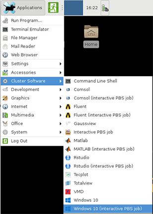
The dialog menus will walk you through setting up and loading your VM.
- You can choose to create a new image or load a saved image.
- New VMs should be saved on Scratch or Research Data Depot as they are too large for Home Directories.
- If you are using scratch, remember that scratch spaces are temporary, and be sure to safely back up your disk image somewhere permanent, such as Research Data Depot or Fortress.
You will also be prompted to select a storage space to mount on your image (Home, Scratch, or Data Depot). You can only choose one to be mounted. It will appear on a shortcut on the desktop once the VM loads.
Link to section 'Notes' of 'Menu Launcher' Notes
Using the menu launcher will launch automatically select reasonable CPU and memory values. If you wish to choose other options or work Windows VMs into scripted workflows see the section on using the command line.
NGC (Nvidia GPU Cloud)
Link to section 'What is NGC?' of 'NGC (Nvidia GPU Cloud)' What is NGC?
Nvidia GPU cloud (NGC) is a GPU-accelerated cloud platform optimized for deep learning and scientific computing. NGC offers a comprehensive catalogue of GPU-accelerated containers, so the application runs quickly and reliably on the high performance computing environment. NGC was deployed to extend the cluster capabilities and to enable powerful software and deliver the fastest results. By utilizing Singularity and NGC, users can focus on building lean models, producing optimal solutions and gathering faster insights. For more information, please visit https://www.nvidia.com/en-us/gpu-cloud and NGC software catalog.
Link to section 'Getting Started' of 'NGC (Nvidia GPU Cloud)' Getting Started
Users can download containers from the NGC software catalog and run them directly using Singularity instructions from the corresponding container’s catalog page.
In addition, a subset of pre-downloaded NGC containers wrapped into convenient software modules are provided. These modules wrap underlying complexity and provide the same commands that are expected from non-containerized versions of each application.
On Scholar, type the command below to see the lists of NGC containers we deployed.
$ module load ngc$ module avail
Link to section 'Example' of 'NGC (Nvidia GPU Cloud)' Example
This example demonstrates how to run LAMMPS with NGC modules.
First, let's prepare the run folder and download the input file for the example we are going to run.
$ cd $CLUSTER_SCRATCH$ mkdir -p lammps_ngc$ cd lammps_ngc$ wget https://lammps.sandia.gov/inputs/in.lj.txt
Then ssh to gpu and load cuda, ngc and lammps modules
$ ssh gpu.scholar.rcac.purdue.edu$ module load cuda$ module load ngc$ module load lammps/29Oct2020
Finally we can set variables and start running lammps.
$ gpu_count=1$ input=in.lj.txt$ mpirun -n ${gpu_count} lmp -k on g ${gpu_count} -sf kk -pk kokkos cuda/aware on neigh full comm device binsize 2.8 -var x 8 -var y 4 -var z 8 -in ${input}
For more information, see each application’s NGC catalog page . For applications deployed as modules, see module help command for direct link to the relevant page (e.g. module help lammps/29Oct2020 in the above example).
BioContainers Collection
Link to section 'What is BioContainers?' of 'BioContainers Collection' What is BioContainers?
The BioContainers project came from the idea of using the containers-based technologies such as Docker or rkt for bioinformatics software. Having a common and controllable environment for running software could help to deal with some of the current problems during software development and distribution. BioContainers is a community-driven project that provides the infrastructure and basic guidelines to create, manage and distribute bioinformatics containers with a special focus on omics fields such as proteomics, genomics, transcriptomics and metabolomics. . For more information, please visit BioContainers project.
Link to section ' Getting Started ' of 'BioContainers Collection' Getting Started
Users can download bioinformatic containers from the BioContainers.pro and run them directly using Singularity instructions from the corresponding container’s catalog page.
Brief Singularity guide and examples are available at the Scholar Singularity user guide page. Detailed Singularity user guide is available at: sylabs.io/guides/3.8/user-guide
In addition, a subset of pre-downloaded biocontainers wrapped into convenient software modules are provided. These modules wrap underlying complexity and provide the same commands that are expected from non-containerized versions of each application.
On Scholar, type the command below to see the lists of biocontainers we deployed.
module load biocontainers
module avail

------------ BioContainers collection modules -------------
      bamtools/2.5.1
      beast2/2.6.3
      bedtools/2.30.0
      blast/2.11.0
      bowtie2/2.4.2
      bwa/0.7.17
      cufflinks/2.2.1
      deeptools/3.5.1
      fastqc/0.11.9
      faststructure/1.0
      htseq/0.13.5
[....]
Link to section ' Example ' of 'BioContainers Collection' Example
This example demonstrates how to run BLASTP with the blast module. This blast module is a biocontainer wrapper for NCBI BLAST.
module load biocontainers
module load blast
blastp -query query.fasta -db nr -out output.txt -outfmt 6 -evalue 0.01
To run a job in batch mode, first prepare a job script that specifies the BioContainer modules you want to launch and the resources required to run it. Then, use the sbatch command to submit your job script to Slurm. The following example shows the job script to use Bowtie2 in bioinformatic analysis.
#!/bin/bash

#SBATCH -A myqueuename
#SBATCH -o bowtie2_%j.txt
#SBATCH -e bowtie2_%j.err
#SBATCH --nodes=1
#SBATCH --ntasks-per-node=1
#SBATCH --cpus-per-task=8
#SBATCH --time=1:30:00
#SBATCH --job-name bowtie2

# Load the Bowtie module
module load biocontainers
module load bowtie2

# Indexing a reference genome
bowtie2-build  ref.fasta ref

# Aligning paired-end reads
bowtie2 -p 8 -x ref -1  reads_1.fq -2 reads_2.fq -S align.sam
To help users get started, we provided detailed user guides for each containerized bioinformatics module on the ReadTheDocs platform
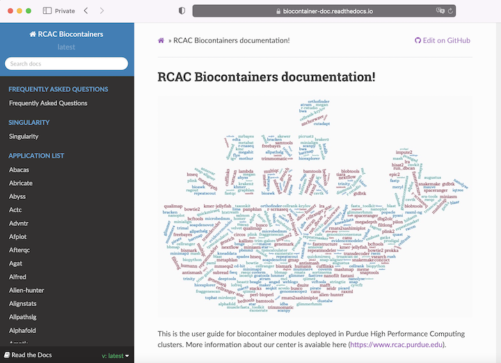
Ansys Fluent
Ansys is a CAE/multiphysics engineering simulation software that utilizes finite element analysis for numerically solving a wide variety of mechanical problems. The software contains a list of packages and can simulate many structural properties such as strength, toughness, elasticity, thermal expansion, fluid dynamics as well as acoustic and electromagnetic attributes.
Link to section 'Ansys Licensing' of 'Ansys Fluent' Ansys Licensing
The Ansys licensing on our community clusters is maintained by Purdue ECN group. There are two types of licenses: teaching and research. For more information, please refer to ECN Ansys licensing page. If you are interested in purchasing your own research license, please send email to software@ecn.purdue.edu.
Link to section 'Ansys Workflow' of 'Ansys Fluent' Ansys Workflow
Ansys software consists of several sub-packages such as Workbench and Fluent. Most simulations are performed using the Ansys Workbench console, a GUI interface to manage and edit the simulation workflow. It requires X11 forwarding for remote display so a SSH client software with X11 support or a remote desktop portal is required. Please see Logging In section for more details. To ensure preferred performance, ThinLinc remote desktop connection is highly recommended.
Typically users break down larger structures into small components in geometry with each of them modeled and tested individually. A user may start by defining the dimensions of an object, adding weight, pressure, temperature, and other physical properties.
Ansys Fluent is a computational fluid dynamics (CFD) simulation software known for its advanced physics modeling capabilities and accuracy. Fluent offers unparalleled analysis capabilities and provides all the tools needed to design and optimize new equipment and to troubleshoot existing installations.
In the following sections, we provide step-by-step instructions to lead you through the process of using Fluent. We will create a classical elbow pipe model and simulate the fluid dynamics when water flows through the pipe. The project files have been generated and can be downloaded via fluent_tutorial.zip.
Link to section 'Loading Ansys Module' of 'Ansys Fluent' Loading Ansys Module
Different versions of Ansys are installed on the clusters and can be listed with module spider or module avail command in the terminal.
$ module avail ansys/
---------------------- Core Applications -----------------------------
   ansys/2019R3    ansys/2020R1    ansys/2021R2    ansys/2022R1 (D)
Before launching Ansys Workbench, a specific version of Ansys module needs to be loaded. For example, you can module load ansys/2021R2 to use the latest Ansys 2021R2. If no version is specified, the default module -> (D) (ansys/2022R1 in this case) will be loaded. You can also check the loaded modules with module list command.
Link to section 'Launching Ansys Workbench' of 'Ansys Fluent' Launching Ansys Workbench
Open a terminal on Scholar, enter rcac-runwb2 to launch Ansys Workbench.
You can also use runwb2 to launch Ansys Workbench. The main difference between runwb2and rcac-runwb2 is that the latter sets the project folder to be in your scratch space. Ansys has an known bug that it might crash when the project folder is set to $HOME on our systems.
Preparing Case Files for Fluent
Link to section 'Creating a Fluent fluid analysis system' of 'Preparing Case Files for Fluent' Creating a Fluent fluid analysis system
In the Ansys Workbench, create a new fluid flow analysis by double-clicking the Fluid Flow (Fluent) option under the Analysis Systems in the Toolbox on the left panel. You can also drag-and-drop the analysis system into the Project Schematic. A green dotted outline indicating a potential location for the new system initially appears in the Project Schematic. When you drag the system to one of the outlines, it turns into a red box to indicate the chosen location of the new system.
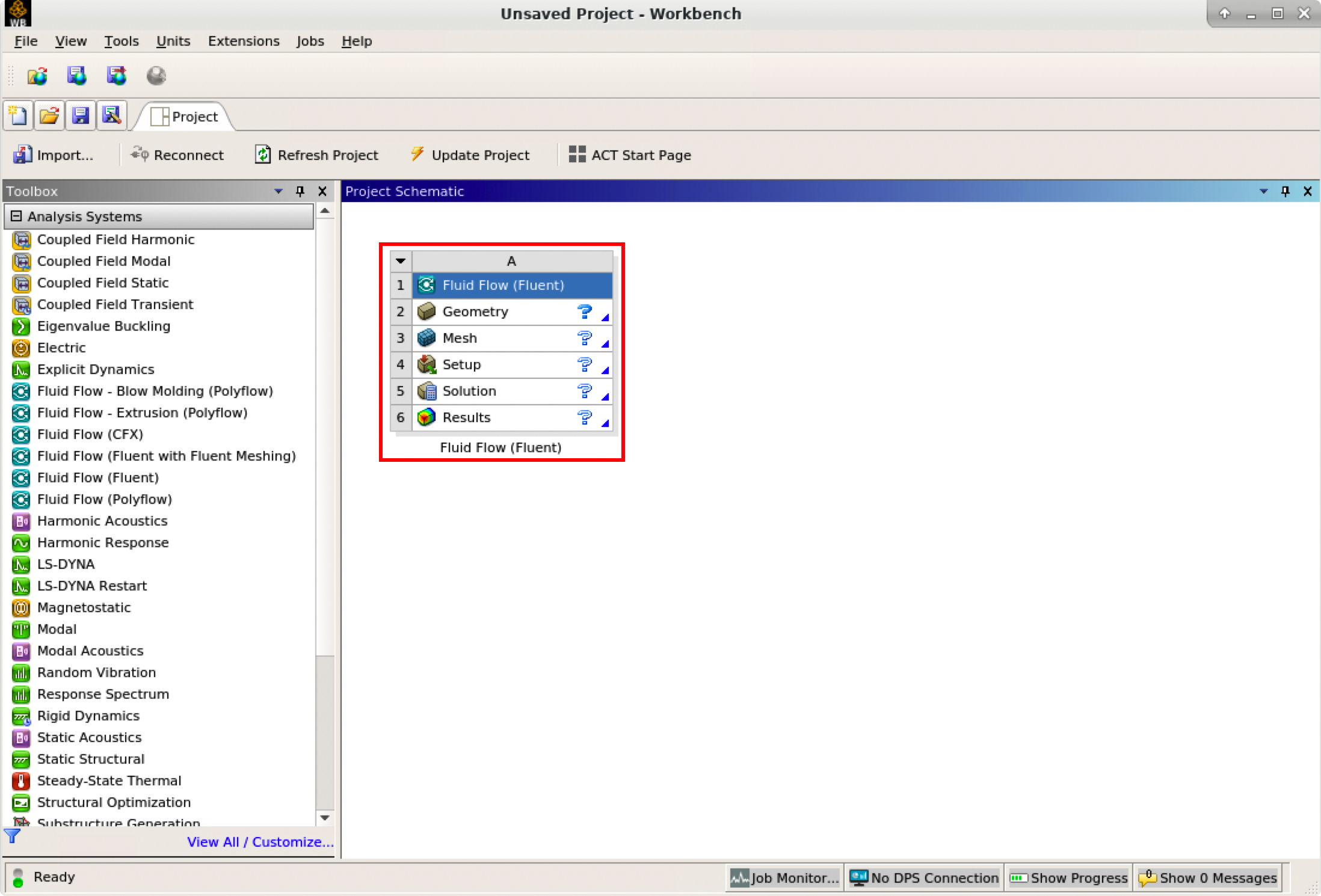
The red rectangle indicates the Fluid Flow system for Fluent, which includes all the essential workflows from “2 Geometry” to “6 Results”. You can rename it and carry out the necessary step-by-step procedures by double-clicking the corresponding cells.
It is important to save the project. Ansys Workbench saves the project with a .wbpj extension and also all the supporting files into a folder with the same name. In this case, a file named elbow_demo.wbpj and a folder $Ansys_PROJECT_FOLDER/elbow_demo_files/ are created in the Ansys project folder:
$ ll
total 33
drwxr-xr-x 7  myusername itap     9 Mar  3 17:47 elbow_demo_files
-rw-r--r-- 1  myusername itap 42597 Mar  3 17:47 elbow_demo.wbpj
You should always “Update Project” and save it after finishing a procedure.
Link to section 'Creating Geometry in the Ansys DesignModeler' of 'Preparing Case Files for Fluent' Creating Geometry in the Ansys DesignModeler
Create a geometry in the Ansys DesignModeler (by double-clicking “Geometry” cell in workflow), or import the appropriate geometry file (by right-clicking the Geometry cell and selecting “Import Geometry” option from the context menu).
You can use Ansys DesignModeler to create 2D/3D geometries or even draw the objects yourself. In our example, we created only half of the elbow pipe because the symmetry of the structure is taken into account to reduce the computation intensity.
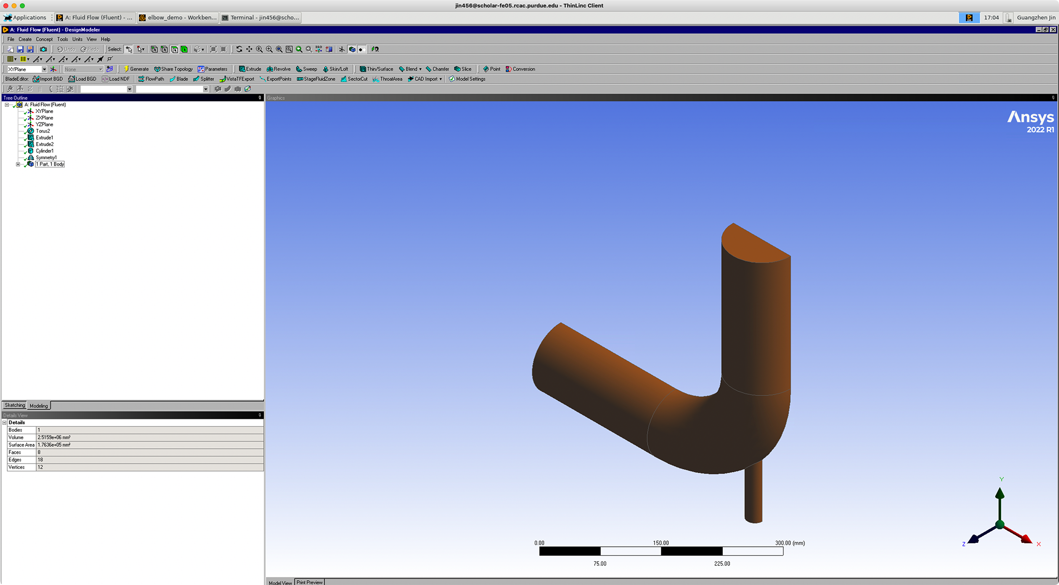
After saving the geometry, a geometry file FFF.agdb will be created in the folder: $Ansys_PROJECT_FOLDER/elbow_demo_file/dp0/FFF/DM/. The project in Workbench will be updated automatically.
If you import a pre-existing geometry into Ansys DesignModeler, it will also generate this file with the same filename at this location.
Link to section 'Creating mesh in the Ansys Meshing' of 'Preparing Case Files for Fluent' Creating mesh in the Ansys Meshing
Now that we have created the elbow pipe geometry, a computational mesh can be generated by the Meshing application throughout the flow volume.
With the successful creation of the geometry, there should be a green check showing the completion of “Geometry” in the Ansys Workbench. A Refresh Required icon within the “Mesh” cell indicates the mesh needs to be updated and refreshed for the system.
Then it’s time to open the Ansys Meshing application by double-clicking the “Mesh” cell and editing the mesh for the project. Generally, there are several steps we need to take to define the mesh:
- Create names for all geometry boundaries such as the inlets, outlets and fluid body. Note: You can use the strings “velocity inlet” and “pressure outlet” in the named selections (with or without hyphens or underscore characters) to allow Ansys Fluent to automatically detect and assign the corresponding boundary types accordingly. Use “Fluid” for the body to let Ansys Fluent automatically detect that the volume is a fluid zone and treat it accordingly.
- Set basic meshing parameters for the Ansys Meshing application. Here are several important parameters you may need to assign: Sizing, Quality, Body Sizing Control, Inflation.
- Select “Generate” to generate the mesh and “Update” to update the mesh into the system. Note: Once the mesh is generated, you can view the mesh statistics by opening the Statistics node in the Details of “Mesh” view. This will display information such as the number of nodes and the number of elements, which gives you a general idea for the future computational resources and time.
After generation and updating the mesh, a mesh file FFF.msh will be generated in folder $Ansys_PROJECT_FOLDER/elbow_demo_file/dp0/FFF/MECH/ and a mesh database file FFF.mshdb will be generated in folder $Ansys_PROJECT_FOLDER/elbow_demo_file/dp0/global/MECH/.
Parameters used in demo case (use default if not assigned):
- Length Unit=”mm”
- Names defined for geometry:
- velocity-inlet-large (large inlet on pipe);
- velocity-inlet-small (small inlet on pipe);
- pressure-outlet (outlet on pipe);
- symmetry (symmetry surface);
- Fluid (body);
- Mesh:
- Quality: Smoothing=”high”;
- Inflation: Use Automatic Inflation=“Program Controlled”, Inflation Option=”Smooth Transition”;
- Statistics:
- Nodes=29371;
- Elements=87647.
Link to section 'Calculation with Fluent' of 'Preparing Case Files for Fluent' Calculation with Fluent
Now all the preparations have been ready for the numerical calculation in Ansys Fluent. Both “Geometry” and “Mesh” cells should have green checks on. We can set up the CFD simulation parameters in Ansys Fluent by double-clicking the “Setup” cell.
When Ansys Fluent is first started or by selecting “editing” on the “Setup” cell, the Fluent Launcher is displayed, enabling you to view and/or set certain Ansys Fluent start-up options (e.g. Precision, Parallel, Display). Note that “Dimension” is fixed to “3D” because we are using a 3D model in this project.
After the Fluent is opened, an Ansys Fluent settings file FFF.set is written under the folder $Ansys_PROJECT_FOLDER/elbow_demo_file/dp0/FFF/Fluent/.
Then we are going to set up all the necessary parameters for Fluent computation. Here are the key steps for the setup:
- Setting up the domain:
- Change the units for length to be consistent with the Mesh;
- Check the mesh statistics and quality;
- Setting up physics:
- Solver: “Energy”, “Viscous Model”, “Near-Wall Treatment”;
- Materials;
- Zones;
- Boundaries: Inlet, Outlet, Internal, Symmetry, Wall;
- Solving:
- Solution Methods;
- Reports;
- Initialization;
- Iterations and output frequency.
Then the calculation will be carried out and the results will be written out into FFF-1.cas.gz under folder $Ansys_PROJECT_FOLDER/elbow_demo_file/dp0/FFF/Fluent/.
This file contains all the settings and simulation results which can be loaded for post analysis and re-computation (more details will be introduced in the following sections). If only configurations and settings within the Fluent are needed, we can open independent Fluent or submit Fluent jobs with bash commands by loading the existing case in order to facilitate the computation process.
Parameters used in demo case (use default if not assigned):
- Domain Setup: Length Units=”mm”;
- Solver: Energy=”on”; Viscous Model=”k-epsilon”; Near-Wall Treatment=”Enhanced Wall Treatment”;
- Materials: water (Density=1000[kg/m^3]; Specific Heat=4216[J/kg-k]; Thermal Conductivity=0.677[w/m-k]; Viscosity=8e-4[kg/m-s]);
- Zones=”fluid (water)”;
- Inlet=”velocity-inlet-large” (Velocity Magnitude=0.4m/s, Specification Method=”Intensity and Hydraulic Diameter”, Turbulent Intensity=5%; Hydraulic Diameter=100mm; Thermal Temperature=293.15k) &”velocity-inlet-small” (Velocity Magnitude=1.2m/s, Specification Method=”Intensity and Hydraulic Diameter”, Turbulent Intensity=5%; Hydraulic Diameter=25mm; Thermal Temperature=313.15k); Internal=”interior-fluid”; Symmetry=”symmetry”; Wall=”wall-fluid”;
- Solution Methods: Gradient=”Green-Gauss Node Based”;
- Report: plot residual and “Facet Maximum” for “pressure-outlet”
- Hybrid Initialization;
- 300 iterations.
Case Calculating with Fluent
Link to section 'Calculation with Fluent' of 'Case Calculating with Fluent' Calculation with Fluent
Now all the files are ready for the Fluent calculations. Both “Geometry” and “Mesh” cells should have green checks. We can set up the CFD simulation parameters in the Ansys Fluent by double-clicking the “Setup” cell.
Ansys Fluent Launcher can be started by selecting “editing” on the “Setup” cell with many startup options (e.g. Precision, Parallel, Display). Note that “Dimension” is fixed to “3D” because we are using a 3D model in this project.
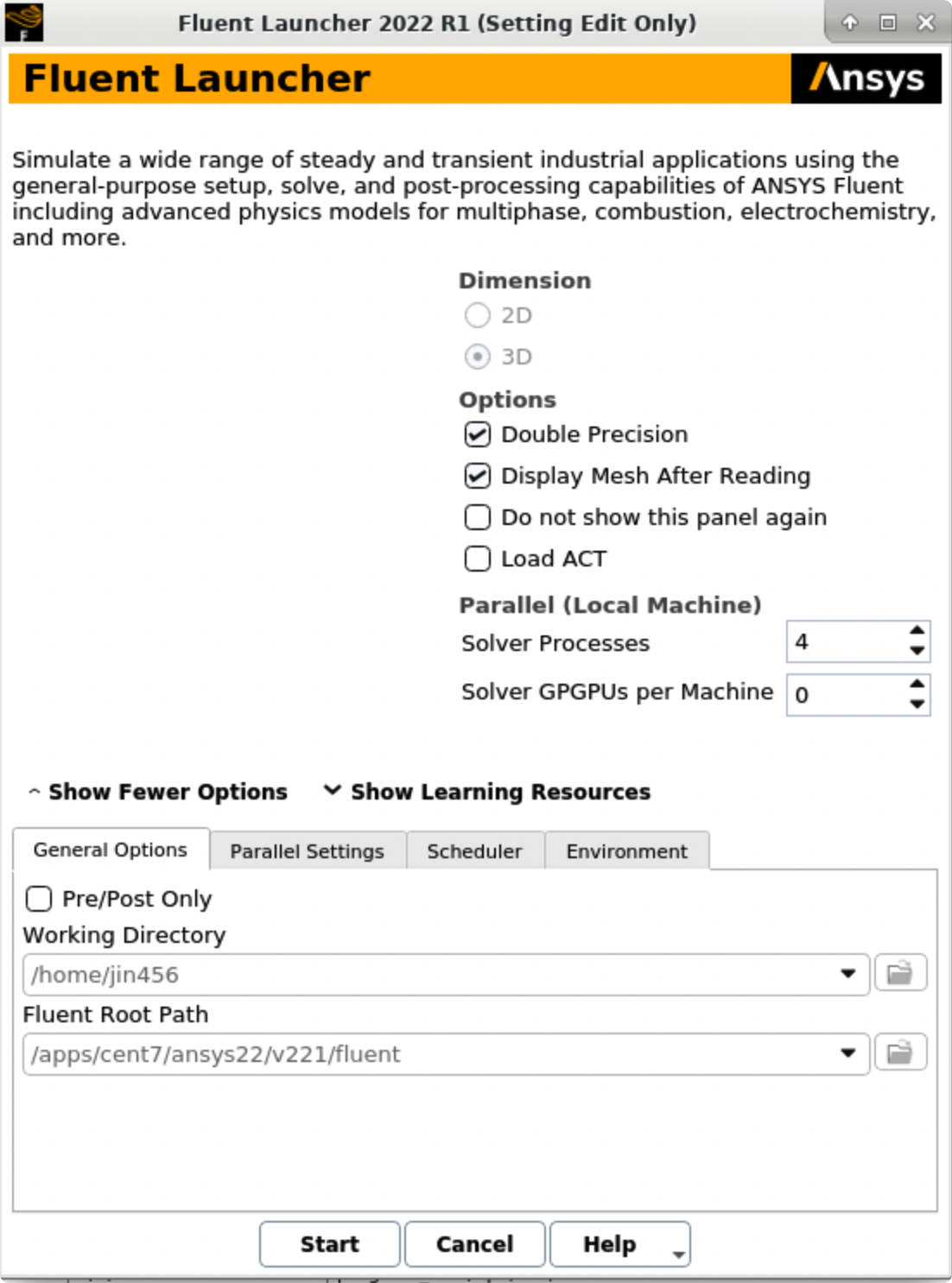
After the Fluent is opened, an Ansys Fluent settings file FFF.set is written under the folder $Ansys_PROJECT_FOLDER/elbow_demo_file/dp0/FFF/Fluent/.
Then we are going to set up all the necessary parameters for Fluent computation. Here are the key steps for the setup:
- Setting up the domain:
- Change the units for length to be consistent with the Mesh;
- Check the mesh statistics and quality;
- Setting up physics:
- Solver: “Energy”, “Viscous Model”, “Near-Wall Treatment”;
- Materials;
- Zones;
- Boundaries: Inlet, Outlet, Internal, Symmetry, Wall;
- Solving:
- Solution Methods;
- Reports;
- Initialization;
- Iterations and output frequency.
Then the calculation will be carried out and the results will be written out into FFF-1.cas.gz under folder $Ansys_PROJECT_FOLDER/elbow_demo_file/dp0/FFF/Fluent/.
This file contains all the settings and simulation results which can be loaded for post analysis and re-computation (more details will be introduced in the following sections). If only configurations and settings within the Fluent are needed, we can open independent Fluent or submit Fluent jobs with bash commands by loading the existing case in order to facilitate the computation process.
Parameters used in demo case (use default if not assigned):
- Domain Setup: Length Units=”mm”;
- Solver: Energy=”on”; Viscous Model=”k-epsilon”; Near-Wall Treatment=”Enhanced Wall Treatment”;
- Materials: water (Density=1000[kg/m^3]; Specific Heat=4216[J/kg-k]; Thermal Conductivity=0.677[w/m-k]; Viscosity=8e-4[kg/m-s]);
- Zones=”fluid (water)”;
- Inlet=”velocity-inlet-large” (Velocity Magnitude=0.4m/s, Specification Method=”Intensity and Hydraulic Diameter”, Turbulent Intensity=5%; Hydraulic Diameter=100mm; Thermal Temperature=293.15k) &”velocity-inlet-small” (Velocity Magnitude=1.2m/s, Specification Method=”Intensity and Hydraulic Diameter”, Turbulent Intensity=5%; Hydraulic Diameter=25mm; Thermal Temperature=313.15k); Internal=”interior-fluid”; Symmetry=”symmetry”; Wall=”wall-fluid”;
- Solution Methods: Gradient=”Green-Gauss Node Based”;
- Report: plot residual and “Facet Maximum” for “pressure-outlet”
- Hybrid Initialization;
- 300 iterations.
Link to section 'Results analysis' of 'Case Calculating with Fluent' Results analysis
The best methods to view and analyze the simulation should be the Ansys Fluent (directly after computation) or the Ansys CFD-Post (entering “Results” in Ansys Workbench). Both methods are straightforward so we will not cover this part in this tutorial. Here is a final simulation result showing the temperature of the symmetry after 300 iterations for reference:

Fluent Text User Interface and Journal File
Link to section 'Fluent Text User Interface (TUI)' of 'Fluent Text User Interface and Journal File' Fluent Text User Interface (TUI)
If you pay attention to the “Console” window in the Fluent window when setting up and carrying out the calculation, corresponding commands can be found and executed one after another. Almost all the setting processes can be accomplished by the command lines, which is called Fluent Text User Interface (TUI). Here are the main commands in Fluent TUI:
  adjoint/                parallel/               solve/
  define/                 plot/                   surface/
  display/                preferences/            turbo-workflow/
  exit                    print-license-usage     views/
  file/                   report/
  mesh/                   server/
For example, instead of opening a case by clicking buttons in Ansys Fluent, we can type /file read-case case_file_name.cas.gz to open the saved case.
Link to section 'Fluent Journal Files' of 'Fluent Text User Interface and Journal File' Fluent Journal Files
A Fluent journal file is a series of TUI commands stored in a text file. The file can be written in a text editor or generated by Fluent as a transcript of the commands given to Fluent during your session.
A journal file generated by Fluent will include any GUI operations (in a TUI form, though). This is quite useful if you have a series of tasks that you need to execute, as it provides a shortcut. To record a journal file, start recording with File -> Write -> Start Journal..., perform whatever tasks you need, and then stop recording with File -> Write -> Stop Journal...
You can also write your own journal file into a text file. The basic rule for a Fluent journal file is to reproduce the TUI commands that controlled the configuration and calculation of Fluent in their order. You can add a comment in a line starting with a ; (semicolon).
Here are some reasons why you should use a Fluent journal file:
- Using journal files with bash scripting can allow you to automate your jobs.
- Using journal files can allow you to parameterize your models easily and automatically.
- Using a journal file can set parameters you do not have in your case file e.g. autosaving.
- Using a journal file can allow you to safely save, stop and restart your jobs easily.
The order of your journal file commands is highly important. The correct sequences must be followed and some stages have multiple options e.g. different initialization methods.
Here is a sample Fluent journal file for the demo case:
  ;testJournal.jou
  ;Set the TUI version for Fluent
  /file/set-tui-version "22.1"
  ;Read the case. The default folder
  /file read-case /home/jin456/Fluent_files/tutorial_case1/elbow_files/dp0/FFF/Fluent/FFF-1.cas.gz
  ;Initialize the case with Hybrid Initialization
  /solve/initialize/hyb-initialization
  ;Set Number of Iterations to 1000, Reporting Interval to 10 iterations and Profile Update Interval to 1 iteration
  /solve/iterate 1000 10 1
  ;Outputting solver performance data upon completion of the simulation
  /parallel timer usage
  ;Write out the simulation results.
  /file write-case-data /home/jin456/Fluent_files/tutorial_case1/elbow_files/dp0/FFF/Fluent/result.cas.h5
  ;After computation, exit Flent
  /exit
Before running this Fluent journal file, you need to make sure: 1) the ansys module has been loaded (it’s highly recommended to load the same version of Ansys when you built the case project); 2) the project case file (***.cas.gz) has been created.
Then we can use Fluent to run this journal file by simply using:fluent 3ddp -t$NTASKS -g -i testJournal.jou in the terminal. Here, 3d indicates this is a 3d model, dp indicates double precision, -t$NTASKS tells Fluent how many Solver Processes it will take (e.g. -t4), -g means to run without the GUI or graphics, -i testJournal.jou tells Fluent to read the specific journal file.
Here is a table for the available command line Options for Linux/UNIX and Windows Platforms in Ansys Fluent.
| Option | Platform | Description |
|---|---|---|
-cc |
all | Use the classic color scheme |
-ccp x |
Windows only | Use the Microsoft Job Scheduler where x is the head node name. |
-cnf=x |
all | Specify the hosts or machine list file |
-driver |
all | Sets the graphics driver (available drivers vary by platform - opengl or x11 or null(Linux/UNIX) - opengl or msw or null (Windows)) |
-env |
all | Show environment variables |
-fgw |
all | Disables the embedded graphics |
-g |
all | Run without the GUI or graphics (Linux/UNIX); Run with the GUI minimized (Windows) |
-gr |
all | Run without graphics |
-gu |
all | Run without the GUI but with graphics (Linux/UNIX); Run with the GUI minimized but with graphics (Windows) |
-help |
all | Display command line options |
-hidden |
Windows only | Run in batch mode |
-host_ip=host:ip |
all | Specify the IP interface to be used by the host process |
-i journal |
all | Reads the specified journal file |
-lsf |
Linux/UNIX only | Run FLUENT using LSF |
-mpi= |
all | Specify MPI implementation |
-mpitest |
all | Will launch an MPI program to collect network performance data |
-nm |
all | Do not display mesh after reading |
-pcheck |
Linux/UNIX only | Checks all nodes |
-post |
all | Run the FLUENT post-processing-only executable |
-p |
all | Choose the interconnect |
-r |
all | List all releases installed |
-rx |
all | Specify release number |
-sge |
Linux/UNIX only | Run FLUENT under Sun Grid Engine |
-sge queue |
Linux/UNIX only | Name of the queue for a given computing grid |
-sgeckpt ckpt_obj |
Linux/UNIX only | Set checkpointing object to ckpt_objfor SGE |
-sgepe fluent_pe min_n-max_n |
Linux/UNIX only | Set the parallel environment for SGE to fluent_pe, min_nand max_n are number of min and max nodes requested |
-tx |
all | Specify the number of processors x |
For more information for Fluent text user interface and journal files, please refer to Fluent FAQ.
Submitting Fluent jobs to SLURM
The Fluent simulations can also run in batch. In this section we provide an example script for submitting Fluent jobs to the SLURM scheduler. Please refer to the Running Jobs section of our user guide for detailed tutorials of submitting jobs.
#!/bin/bash
# Job script for submitting a FLUENT job on multiple cores on a single node

# Apply resources via SLURM
#SBATCH --nodes=1
#SBATCH --ntasks=4
#SBATCH --time=01:00:00
#SBATCH --job-name=fluent_test
#SBATCH -o fluent_test_%j.out
#SBATCH -e fluent_test_%j.err

# Loads Ansys and sets the application up
module purge
module load ansys/2022R1

#Initiating Fluent and reading input journal file
fluent 3ddp -t$NTASKS -g -i testJournal.jou
For more information about submitting Fluent jobs, please refer to Fluent FAQ .
Using Jupyter Hub on Scholar
JupyterHub is a multi-user Hub that spawns, manages, and proxies multiple instances of the single-user Jupyter notebook server. JupyterHub can be used to serve notebooks to a class of students, a corporate data science group, or a scientific research group.
Users can use the Open OnDemand (https://gateway.scholar.rcac.purdue.edu/) portal to launch private Jupyter servers on the Scholar compute nodes. OOD provides a browser-based interface to launch and run Jupyter notebooks. The old centralized Jupyter server has been deprecated with Scholar's OS upgrade in Dec 2024.
Frequently Asked Questions
Some common questions, errors, and problems are categorized below. Click the Expand Topics link in the upper right to see all entries at once. You can also use the search box above to search the user guide for any issues you are seeing.
About Scholar
Frequently asked questions about Scholar.
Can you remove me from the Scholar mailing list?
Your subscription in the Scholar mailing list is tied to your account on Scholar. If you are no longer using your account on Scholar, your account can be deleted from the My Accounts page. Hover over the resource you wish to remove yourself from and click the red 'X' button. Your account and mailing list subscription will be removed overnight. Be sure to make a copy of any data you wish to keep first.
How is Scholar different than other Community Clusters?
Scholar differs from other Community Clusters in many significant aspects:
- Scholar is a hybrid cluster for teaching courses that require high-performance computing.
- A subset of Scholar front-ends contain Nvidia Tesla V100 accelerator cards. You can access these front ends by logging in to
gpu.scholar.rcac.purdue.edu. - A subset of Scholar compute nodes contain Nvidia Tesla V100 accelerator cards which can significantly improve performance of compute-intensive workloads. These can be utilized by submitting jobs to the gpu queue (add -A gpu to your job submission command).
- A selection of GPU-enabled application containers from the Nvidia GPU Cloud (NGC) collection is installed.
Do I need to do anything to my firewall to access Scholar?
No firewall changes are needed to access Scholar. However, to access data through Network Drives (i.e., CIFS, "Z: Drive"), you must be on a Purdue campus network or connected through VPN.
Does Scholar have the same home directory as other clusters?
The Scholar home directory and its contents are exclusive to Scholar cluster front-end hosts and compute nodes. This home directory is not available on other RCAC machines but Scholar. There is no automatic copying or synchronization between home directories.
At your discretion you can manually copy all or parts of your main research computing home to Scholar using one of the suggested methods.
If you plan to use hsi or htar commands to access Fortress tape archive from Scholar, please see also the keytab generation question for a temporary workaround to a potential caveat, while a permanent mitigation is being developed.
Logging In & Accounts
Frequently asked questions about logging in & accounts.
Errors
Common errors and solutions/work-arounds for them.
/usr/bin/xauth: error in locking authority file
Link to section 'Problem' of '/usr/bin/xauth: error in locking authority file' Problem
I receive this message when logging in:
/usr/bin/xauth: error in locking authority file
Link to section 'Solution' of '/usr/bin/xauth: error in locking authority file' Solution
Your home directory disk quota is full. You may check your quota with myquota.
You will need to free up space in your home directory.
ncdu command is a convenient interactive tool to examine disk usage. Consider running ncdu $HOME to analyze where the bulk of the usage is. With this knowledge, you could then archive your data elsewhere (e.g. your research group's Data Depot space, or Fortress tape archive), or delete files you no longer need.
There are several common locations that tend to grow large over time and are merely cached downloads. The following are safe to delete if you see them in the output of ncdu $HOME:
/home/myusername/.local/share/Trash
/home/myusername/.cache/pip
/home/myusername/.conda/pkgs
/home/myusername/.singularity/cache
My SSH connection hangs
Link to section 'Problem' of 'My SSH connection hangs' Problem
Your console hangs while trying to connect to a RCAC Server.
Link to section 'Solution' of 'My SSH connection hangs' Solution
This can happen due to various reasons. Most common reasons for hanging SSH terminals are:
- Network: If you are connected over wifi, make sure that your Internet connection is fine.
- Busy front-end server: When you connect to a cluster, you SSH to one of the front-end login nodes. Due to transient user loads, one or more of the front-ends may become unresponsive for a short while. To avoid this, try reconnecting to the cluster or wait until the login node you have connected to has reduced load.
- File system issue: If a server has issues with one or more of the file systems (
home,scratch, ordepot) it may freeze your terminal. To avoid this you can connect to another front-end.
If neither of the suggestions above work, please contact support specifying the name of the server where your console is hung.
Thinlinc session frozen
Link to section 'Problem' of 'Thinlinc session frozen' Problem
Your Thinlinc session is frozen and you can not launch any commands or close the session.
Link to section 'Solution' of 'Thinlinc session frozen' Solution
This can happen due to various reasons. The most common reason is that you ran something memory-intensive inside that Thinlinc session on a front-end, so parts of the Thinlinc session got killed by Cgroups, and the entire session got stuck.
- If you are using a web-version Thinlinc remote desktop (inside the browser):
The web version does not have the capability to kill the existing session, only the standalone client does. Please install the standalone client and follow the steps below:
- If you are using a Thinlinc client:
Close the ThinLinc client, reopen the client login popup, and select
End existing session.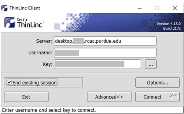
Select "End existing session" and try "Connect" again.
Thinlinc session unreachable
Link to section 'Problem' of 'Thinlinc session unreachable' Problem
When trying to login to Thinlinc and re-connect to your existing session, you receive an error "Your Thinlinc session is currently unreachable".
Link to section 'Solution' of 'Thinlinc session unreachable' Solution
This can happen if the specific login node your existing remote desktop session was residing on is currently offline or down, so Thinlinc can not reconnect to your existing session. Most often the session is non-recoverable at this point, so the solution is to terminate your existing Thinlinc desktop session and start a new one.
- If you are using a web-version Thinlinc remote desktop (inside the browser):
The web version does not have the capability to kill the existing session, only the standalone client does. Please install the standalone client and follow the steps below:
- If you are using a Thinlinc client:
Close the ThinLinc client, reopen the client login popup, and select
End existing session.
Select "End existing session" and try "Connect" again.
How to disable Thinlinc screensaver
Link to section 'Problem' of 'How to disable Thinlinc screensaver' Problem
Your ThinLinc desktop is locked after being idle for a while, and it asks for a password to refresh it. It means the "screensaver" and "lock screen" functions are turned on, but you want to disable these functions.
Link to section 'Solution' of 'How to disable Thinlinc screensaver' Solution
If your screen is locked, close the ThinLinc client, reopen the client login popup, and select End existing session.
To permanently avoid screen lock issue, right click desktop and select Applications, then settings, and select Screensaver.
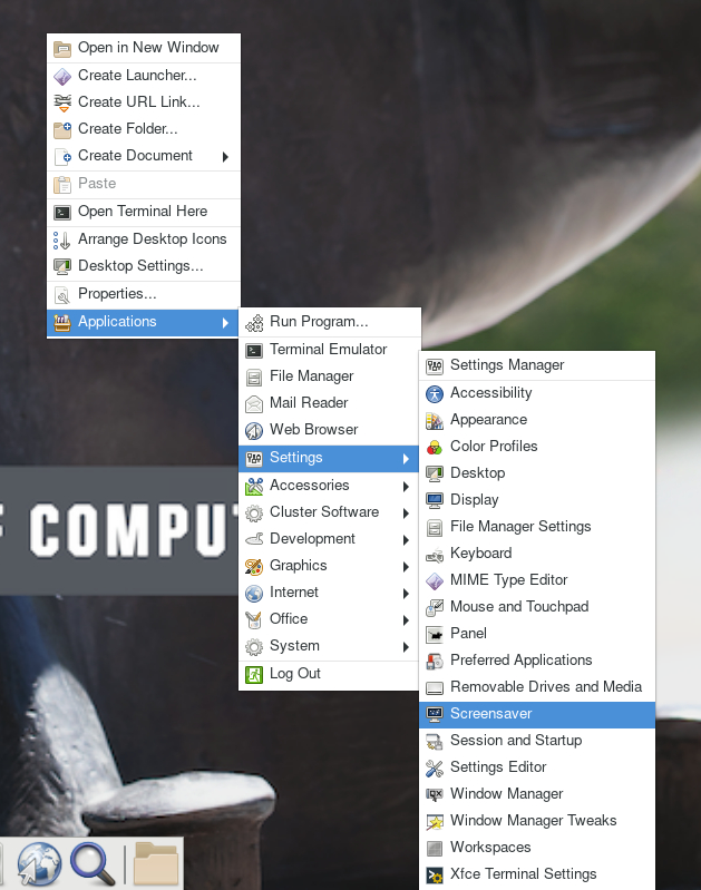
Under Screensaver, turn off the Enable Screensaver, then under Lock Screen, turn off the Enable Lock Screen, and close the window.
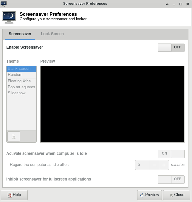
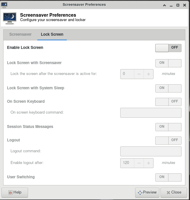
Questions
Frequently asked questions about logging in & accounts.
I worked on Scholar after I graduated/left Purdue, but can not access it anymore
Link to section 'Problem' of 'I worked on Scholar after I graduated/left Purdue, but can not access it anymore' Problem
You have graduated or left Purdue but continue collaboration with your Purdue colleagues. You find that your access to Purdue resources has suddenly stopped and your password is no longer accepted.
Link to section 'Solution' of 'I worked on Scholar after I graduated/left Purdue, but can not access it anymore' Solution
Access to all resources depends on having a valid Purdue Career Account. Expired Career Accounts are removed twice a year, during Spring and October breaks (more details at the official page). If your Career Account was purged due to expiration, you will not be be able to access the resources.
To provide remote collaborators with valid Purdue credentials, the University provides a special procedure called Request for Privileges (R4P). If you need to continue your collaboration with your Purdue PI, the PI will have to submit or renew an R4P request on your behalf.
After your R4P is completed and Career Account is restored, please note two additional necessary steps:
-
Access: Restored Career Accounts by default do not have any RCAC resources enabled for them. Your PI will have to login to the Manage Users tool and explicitly re-enable your access by un-checking and then ticking back checkboxes for desired queues/Unix groups resources.
-
Email: Restored Career Accounts by default do not have their @purdue.edu email service enabled. While this does not preclude you from using RCAC resources, any email messages (be that generated on the clusters, or any service announcements) would not be delivered - which may cause inconvenience or loss of compute jobs. To avoid this, we recommend setting your restored @purdue.edu email service to "Forward" (to an actual address you read). The easiest way to ensure it is to go through the Account Setup process.
Jobs
Frequently asked questions related to running jobs.
Errors
Common errors and potential solutions/workarounds for them.
cannot connect to X server / cannot open display
Link to section 'Problem' of 'cannot connect to X server / cannot open display' Problem
You receive the following message after entering a command to bring up a graphical window
cannot connect to X server cannot open display
Link to section 'Solution' of 'cannot connect to X server / cannot open display' Solution
This can happen due to multiple reasons:
- Reason: Your SSH client software does not support graphical display by itself (e.g. SecureCRT or PuTTY).
- Solution: Try using a client software like Thinlinc or MobaXterm as described in the SSH X11 Forwarding guide.
-
Reason: You did not enable X11 forwarding in your SSH connection.
-
Solution: If you are in a Windows environment, make sure that X11 forwarding is enabled in your connection settings (e.g. in MobaXterm or PuTTY). If you are in a Linux environment, try
ssh -Y -l username hostname
-
- Reason: If you are trying to open a graphical window within an interactive PBS job, make sure you are using the
-Xoption withqsubafter following the previous step(s) for connecting to the front-end. Please see the example in the Interactive Jobs guide. - Reason: If none of the above apply, make sure that you are within quota of your home directory.
bash: command not found
Link to section 'Problem' of 'bash: command not found' Problem
You receive the following message after typing a command
bash: command not found
Link to section 'Solution' of 'bash: command not found' Solution
This means the system doesn't know how to find your command. Typically, you need to load a module to do it.
bash: module command not found
Link to section 'Problem' of 'bash: module command not found' Problem
You receive the following message after typing a command, e.g. module load intel
bash: module command not found
Link to section 'Solution' of 'bash: module command not found' Solution
The system cannot find the module command. You need to source the modules.sh file as below
source /etc/profile.d/modules.sh
or
#!/bin/bash -i
Close Firefox / Firefox is already running but not responding
Link to section 'Problem' of 'Close Firefox / Firefox is already running but not responding' Problem
You receive the following message after trying to launch Firefox browser inside your graphics desktop:
Close Firefox

Firefox is already running, but not responding.  To open a new window,
you  must first close the existing Firefox process, or restart your system.
Link to section 'Solution' of 'Close Firefox / Firefox is already running but not responding' Solution
When Firefox runs, it creates several lock files in the Firefox profile directory (inside ~/.mozilla/firefox/ folder in your home directory). If a newly-started Firefox instance detects the presence of these lock files, it complains.
This error can happen due to multiple reasons:
- Reason: You had a single Firefox process running, but it terminated abruptly without a chance to clean its lock files (e.g. the job got terminated, session ended, node crashed or rebooted, etc).
- Solution: If you are certain you do not have any other Firefox processes running elsewhere, please use the following command in a terminal window to detect and remove the lock files:
$ unlock-firefox
- Solution: If you are certain you do not have any other Firefox processes running elsewhere, please use the following command in a terminal window to detect and remove the lock files:
- Reason: You may indeed have another Firefox process (in another Thinlinc or Gateway session on this or other cluster, another front-end or compute node). With many clusters sharing common home directory, a running Firefox instance on one can affect another.
- Solution: Try finding and closing running Firefox process(es) on other nodes and clusters.
- Solution: If you must have multiple Firefoxes running simultaneously, you may be able to create separate Firefox profiles and select which one to use for each instance.
Jupyter: database is locked / can not load notebook format
Link to section 'Problem' of 'Jupyter: database is locked / can not load notebook format' Problem
You receive the following message after trying to load existing Jupyter notebooks inside your JupyterHub session:
Error loading notebook

An unknown error occurred while loading this notebook.  This version can load notebook formats or earlier. See the server log for details.
Alternatively, the notebook may open but present an error when creating or saving a notebook:
Autosave Failed!

Unexpected error while saving file:  MyNotebookName.ipynb database is locked
Link to section 'Solution' of 'Jupyter: database is locked / can not load notebook format' Solution
When Jupyter notebooks are opened, the server keeps track of their state in an internal database (located inside ~/.local/share/jupyter/ folder in your home directory). If a Jupyter process gets terminated abruptly (e.g. due to an out-of-memory error or a host reboot), the database lock is not cleared properly, and future instances of Jupyter detect the lock and complain.
Please follow these steps to resolve:
- Fully exit from your existing Jupyter session (close all notebooks, terminate Jupyter, log out from JupyterHub or JupyterLab, terminate OnDemand gateway's Jupyter app, etc).
- In a terminal window (SSH, Thinlinc or OnDemand gateway's terminal app) use the following command to clean up stale database locks:
$ unlock-jupyter - Start a new Jupyter session as usual.
Questions
Frequently asked questions about jobs.
How do I know Non-uniform Memory Access (NUMA) layout on Scholar?
- You can learn about processor layout on Scholar nodes using the following command:
scholar-a003:~$ lstopo-no-graphics - For detailed IO connectivity:
scholar-a003:~$ lstopo-no-graphics --physical --whole-io - Please note that NUMA information is useful for advanced MPI/OpenMP/GPU optimizations. For most users, using default NUMA settings in MPI or OpenMP would give you the best performance.
Why cannot I use --mem=0 when submitting jobs?
Link to section 'Question' of 'Why cannot I use --mem=0 when submitting jobs?' Question
Why can't I specify --mem=0 for my job?
Link to section 'Answer' of 'Why cannot I use --mem=0 when submitting jobs?' Answer
We no longer support requesting unlimited memory (--mem=0) as it has an adverse effect on the way scheduler allocates job, and could lead to large amount of nodes being blocked from usage.
Most often we suggest relying on default memory allocation (cluster-specific). But if you have to request custom amounts of memory, you can do it explicitly. For example --mem=20G.
If you want to use the entire node's memory, you can submit the job with the --exclusive option.
Can I extend the walltime on a job?
In some circumstances, yes. Walltime extensions must be requested of and completed by staff. Walltime extension requests will be considered on named (your advisor or research lab) queues. Standby or debug queue jobs cannot be extended.
Extension requests are at the discretion of staff based on factors such as any upcoming maintenance or resource availability. Jobs in the the 'scholar' queue on Scholar cannot be extended. 'Long' queue jobs can be extended to the maximum for that queue.
Please be mindful of time remaining on your job when making requests and make requests at least 24 hours before the end of your job AND during business hours. We cannot guarantee jobs will be extended in time with less than 24 hours notice, after-hours, during weekends, or on a holiday.
We ask that you make accurate walltime requests during job submissions. Accurate walltimes will allow the job scheduler to efficiently and quickly schedule jobs on the cluster. Please consider that extensions can impact scheduling efficiency for all users of the cluster.
Requests can be made by contacting support. We ask that you:
- Provide numerical job IDs, cluster name, and your desired extension amount.
- Provide at least 24 hours notice before job will end (more if request is made on a weekend or holiday).
- Consider making requests during business hours. We may not be able to respond in time to requests made after-hours, on a weekend, or on a holiday.
Data
Frequently asked questions about data and data management.
How is my Data Secured on Scholar?
Scholar is operated in line with policies, standards, and best practices as described within Secure Purdue, and specific to RCAC Resources.
Security controls for Scholar are based on ones defined in NIST cybersecurity standards.
Scholar supports research at the L1 fundamental and L2 sensitive levels. Scholar is not approved for storing data at the L3 restricted (covered by HIPAA) or L4 Export Controlled (ITAR), or any Controlled Unclassified Information (CUI).
For resources designed to support research with heightened security requirements, please look for resources within the REED+ Ecosystem.
Link to section 'For additional information' of 'How is my Data Secured on Scholar?' For additional information
Log in with your Purdue Career Account.
Can I share data with outside collaborators?
Yes! Globus allows convenient sharing of data with outside collaborators. Data can be shared with collaborators' personal computers or directly with many other computing resources at other institutions. See the Globus documentation on how to share data:
Does Scholar have the same home directory as other clusters?
The Scholar home directory and its contents are exclusive to Scholar cluster front-end hosts and compute nodes. This home directory is not available on other RCAC machines but Scholar. There is no automatic copying or synchronization between home directories.
At your discretion you can manually copy all or parts of your main research computing home to Scholar using one of the suggested methods.
If you plan to use hsi or htar commands to access Fortress tape archive from Scholar, please see also the keytab generation question for a temporary workaround to a potential caveat, while a permanent mitigation is being developed.
HSI/HTAR: Unable to authenticate user with remote gateway (error 2 or 9)
There could be a variety of such errors, with wordings along the lines of
Could not initialize keytab on remote server.
result = -2, errno = 2rver connection
*** hpssex_OpenConnection: Unable to authenticate user with remote gateway at 128.211.138.40.1217result = -2, errno = 9
Unable to setup communication to HPSS...
ERROR (main) unable to open remote gateway server connection
HTAR: HTAR FAILED
and
*** hpssex_OpenConnection: Unable to authenticate user with remote gateway at 128.211.138.40.1217result = -11000, errno = 9
Unable to setup communication to HPSS...
*** HSI: error opening logging
Error - authentication/initialization failed
The root cause for these errors is an expired or non-existent keytab file (a special authentication token stored in your home directory). These keytabs are valid for 90 days and on most RCAC resources they are usually automatically checked and regenerated when you execute hsi or htar commands. However, if the keytab is invalid, or fails to generate, Fortress may be unable to authenticate you and you would see the above errors. This is especially common on those RCAC clusters that have their own dedicated home directories (such as Bell), or on standalone installations (such as if you downloaded and installed HSI and HTAR on your non-RCAC computer).
This is a temporary problem and a permanent system-wide solution is being developed. In the interim, the recommended workaround is to generate a new valid keytab file in your main research computing home directory, and then copy it to your home directory on Scholar. The fortresskey command is used to generate the keytab and can be executed on another cluster or a dedicated data management host data.rcac.purdue.edu:
$ ssh myusername@data.rcac.purdue.edu fortresskey
$ scp -pr myusername@data.rcac.purdue.edu:~/.private $HOME
With a valid keytab in place, you should then be able to use hsi and htar commands to access Fortress from Scholar. Note that only one keytab can be valid at any given time (i.e. if you regenerated it, you may have to copy the new keytab to all systems that you intend to use hsi or htar from if they do not share the main research computing home directory).
Can I access Fortress from Scholar?
Yes. While Fortress directories are not directly mounted on Scholar for performance and archival protection reasons, they can be accessed from Scholar front-ends and nodes using any of the recommended methods of HSI, HTAR or Globus.
Software
Frequently asked questions about software.
Cannot use pip after loading ml-toolkit modules
Link to section 'Question' of 'Cannot use pip after loading ml-toolkit modules' Question
Pip throws an error after loading the machine learning modules. How can I fix it?
Link to section 'Answer' of 'Cannot use pip after loading ml-toolkit modules' Answer
Machine learning modules (tensorflow, pytorch, opencv etc.) include a version of pip that is newer than the one installed with Anaconda. As a result it will throw an error when you try to use it.
$ pip --version
Traceback (most recent call last):
  File "/apps/cent7/anaconda/5.1.0-py36/bin/pip", line 7, in <module>
    from pip import main
ImportError: cannot import name 'main'
The preferred way to use pip with the machine learning modules is to invoke it via Python as shown below.
$ python -m pip --version
How can I get access to Sentaurus software?
Link to section 'Question' of 'How can I get access to Sentaurus software?' Question
How can I get access to Sentaurus tools for micro- and nano-electronics design?
Link to section 'Answer' of 'How can I get access to Sentaurus software?' Answer
Sentaurus software license requires a signed NDA. Please contact Dr. Mark Johnson, Director of ECE Instructional Laboratories to complete the process.
Once the licensing process is complete and you have been added into a cae2 Unix group, you could use Sentaurus on RCAC community clusters by loading the corresponding environment module:
module load sentaurus
Julia package installation
Users do not have write permission to the default julia package installation destination. However, users can install packages into home directory under ~/.julia.
Users can side step this by explicitly defining where to put julia packages:
$ export JULIA_DEPOT_PATH=$HOME/.julia
$ julia -e 'using Pkg; Pkg.add("PackageName")'
About Research Computing
Frequently asked questions about RCAC.
Can I get a private server from RCAC?
Link to section 'Question' of 'Can I get a private server from RCAC?' Question
Can I get a private (virtual or physical) server from RCAC?
Link to section 'Answer' of 'Can I get a private server from RCAC?' Answer
Often, researchers may want a private server to run databases, web servers, or other software. RCAC currently has Geddes, a Community Composable Platform optimized for composable, cloud-like workflows that are complementary to the batch applications run on Community Clusters. Funded by the National Science Foundation under grant OAC-2018926, Geddes consists of Dell Compute nodes with two 64-core AMD Epyc 'Rome' processors (128 cores per node).
To purchase access to Geddes today, go to the Cluster Access Purchase page. Please subscribe to our Community Cluster Program Mailing List to stay informed on the latest purchasing developments or contact us (rcac-cluster-purchase@lists.purdue.edu) if you have any questions.
Datasets
Please refer to our Federated Datasets Documentation website for up-to-date datasets on Anvil and instructions on how to use them.